MUMmerplots with ggplot2
Sep 19 2017 R plotUpdate Oct 28 2018: added reference id (rid) to be able to visualize multiple reference regions. Also uploaded the example data somewhere.
library(dplyr)
library(magrittr)
library(GenomicRanges)
library(knitr)
library(ggplot2)
library(tidyr)
MUMmer plot
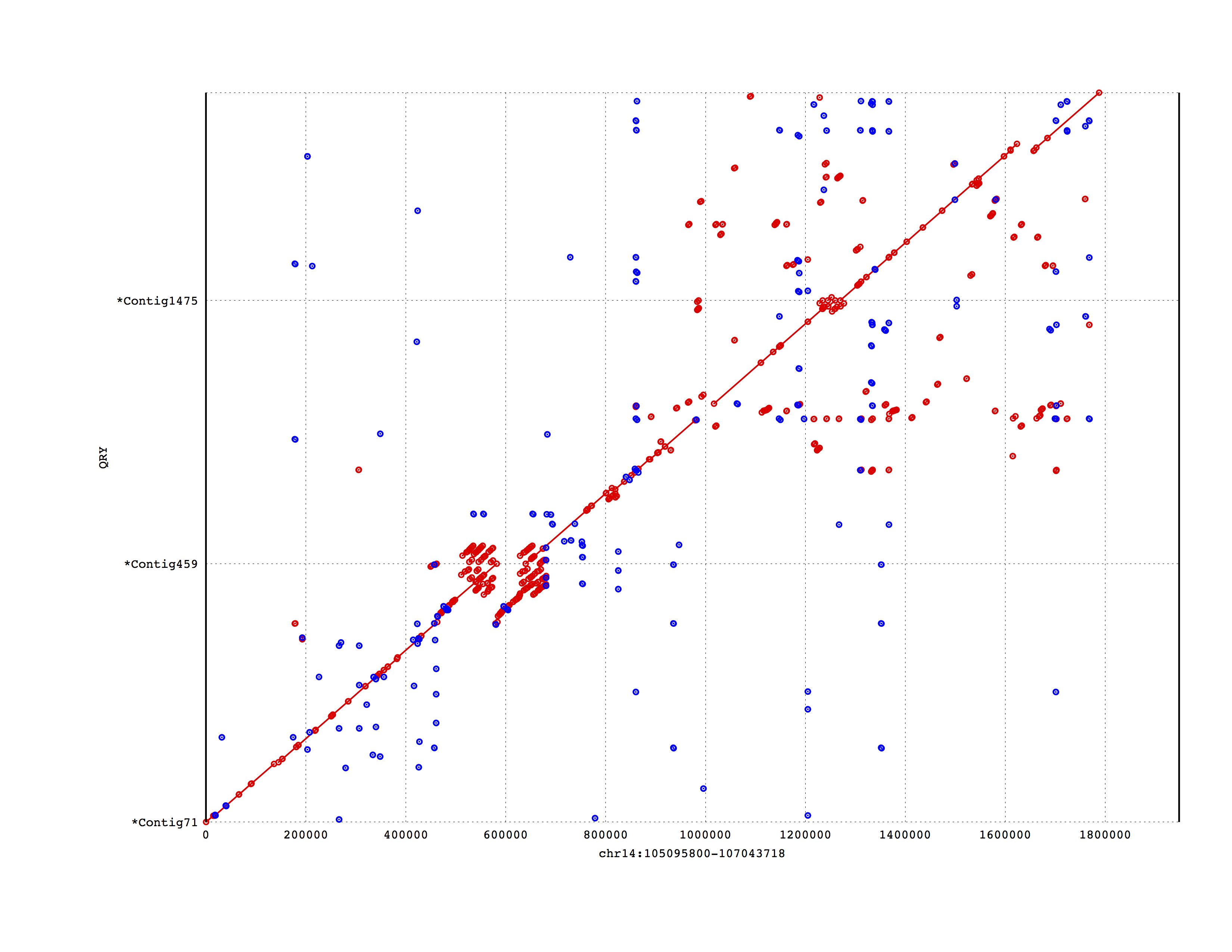
The MUMmer plot that I want to reproduce showed three contigs overlapping a region of chr 14. I had filtered the delta file with delta-filter -l 10000 -q -r to get only the contigs with the best alignments. I had used mummerplot with the -l layout option to reorder and orient the sequences to have a nice diagonal.
Delta file
The delta file is the default output of the NUCmer alignment script. The format of the delta file is described more here.
The delta file used in this post can be downloaded here. Otherwise, in R:
if(!file.exists('mumplot-example.delta')){
    download.file('https://dl.dropboxusercontent.com/s/3zscsbbex6rgemo/mumplot-example.delta?dl0',
                  'mumplot-example.delta')
}
Read a delta file
readDelta <- function(deltafile){
  lines = scan(deltafile, 'a', sep='\n', quiet=TRUE)
  lines = lines[-1]
  lines.l = strsplit(lines, ' ')
  lines.len = lapply(lines.l, length) %>% as.numeric
  lines.l = lines.l[lines.len != 1]
  lines.len = lines.len[lines.len != 1]
  head.pos = which(lines.len == 4)
  head.id = rep(head.pos, c(head.pos[-1], length(lines.l)+1)-head.pos)
  mat = matrix(as.numeric(unlist(lines.l[lines.len==7])), 7)
  res = as.data.frame(t(mat[1:5,]))
  colnames(res) = c('rs','re','qs','qe','error')
  res$qid = unlist(lapply(lines.l[head.id[lines.len==7]], '[', 2))
  res$rid = unlist(lapply(lines.l[head.id[lines.len==7]], '[', 1)) %>% gsub('^>', '', .)
  res$strand = ifelse(res$qe-res$qs > 0, '+', '-')
  res
}

mumgp = readDelta("mumplot-example.delta")

mumgp %>% head %>% kable| rs | re | qs | qe | error | qid | rid | strand |
|---|---|---|---|---|---|---|---|
| 265577 | 265842 | 108520 | 108254 | 46 | Contig0 | chr14:105095800-107043718 | - |
| 265577 | 265842 | 106438 | 106172 | 46 | Contig0 | chr14:105095800-107043718 | - |
| 306695 | 306968 | 138241 | 138515 | 31 | Contig0 | chr14:105095800-107043718 | + |
| 1016956 | 1017364 | 27806 | 27394 | 62 | Contig0 | chr14:105095800-107043718 | - |
| 1723715 | 1723990 | 34123 | 33845 | 26 | Contig0 | chr14:105095800-107043718 | - |
| 1767531 | 1767813 | 33842 | 34123 | 24 | Contig0 | chr14:105095800-107043718 | + |
Filter contigs with poor alignments
For now, I filter contigs simply based on the size of the aligned segment. I keep only contigs with at least one aligned segment larger than a minimum size. Smaller alignment in these contigs are kept if in the same range as the large aligned segments. Eventually, I could also filter segment based on the number/proportion of errors.
filterMum <- function(df, minl=1000, flanks=1e4){
    coord = df %>% filter(abs(re-rs)>minl) %>% group_by(qid, rid) %>%
        summarize(qsL=min(qs)-flanks, qeL=max(qe)+flanks, rs=median(rs)) %>%
        ungroup %>% arrange(desc(rs)) %>%
        mutate(qid=factor(qid, levels=unique(qid))) %>% select(-rs)
    merge(df, coord) %>% filter(qs>qsL, qe<qeL) %>%
        mutate(qid=factor(qid, levels=levels(coord$qid))) %>% select(-qsL, -qeL)
}

mumgp.filt = filterMum(mumgp, minl=1e4)
mumgp.filt %>% head %>% kable| qid | rid | rs | re | qs | qe | error | strand |
|---|---|---|---|---|---|---|---|
| Contig1475 | chr14:105095800-107043718 | 1663946 | 1665485 | 331648 | 330113 | 171 | - |
| Contig1475 | chr14:105095800-107043718 | 1662200 | 1684396 | 126037 | 103837 | 234 | - |
| Contig1475 | chr14:105095800-107043718 | 1581333 | 1582738 | 244635 | 243233 | 87 | - |
| Contig1475 | chr14:105095800-107043718 | 1597381 | 1610746 | 145948 | 132626 | 157 | - |
| Contig1475 | chr14:105095800-107043718 | 1610278 | 1623358 | 130561 | 117468 | 200 | - |
| Contig1475 | chr14:105095800-107043718 | 1616542 | 1618080 | 331648 | 330113 | 146 | - |
Graph
I’m going for the same style as mummerplot to compare.
ggplot(mumgp.filt, aes(x=rs, xend=re, y=qs, yend=qe, colour=strand)) + geom_segment() +
    geom_point(alpha=.5) + facet_grid(qid~., scales='free', space='free', switch='y') +
    theme_bw() + theme(strip.text.y=element_text(angle=180, size=5),
                       legend.position=c(.99,.01), legend.justification=c(1,0),
                       strip.background=element_blank(),
                       axis.text.y=element_blank(), axis.ticks.y=element_blank()) +
    xlab('reference sequence') + ylab('assembly') + scale_colour_brewer(palette='Set1')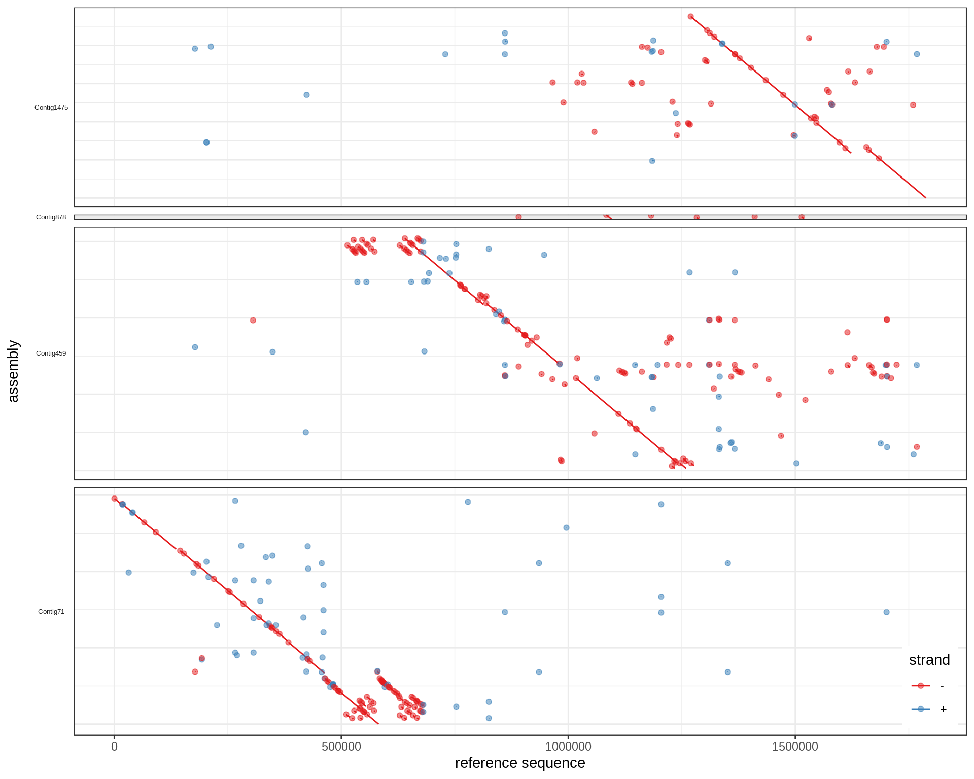
Not bad but it would look nicer if we flipped the contigs to have more or less a diagonal.
Diagonalize
For each contig, I compute the major strand (strand with most bases aligned) and flip if necessary. The contigs are also ordered based on the reference region with most bases and the weighted means of the start position in this matched reference region.
diagMum <- function(df){
    ## Find best qid order
    rid.o = df %>% group_by(qid, rid) %>% summarize(base=sum(abs(qe-qs)),
                                                    rs=weighted.mean(rs, abs(qe-qs))) %>%
        ungroup %>% arrange(desc(base)) %>% group_by(qid) %>% do(head(., 1)) %>%
        ungroup %>% arrange(desc(rid), desc(rs)) %>%
        mutate(qid=factor(qid, levels=unique(qid)))
    ## Find best qid strand
    major.strand = df %>% group_by(qid) %>%
        summarize(major.strand=ifelse(sum(sign(qe-qs)*abs(qe-qs))>0, '+', '-'),
                  maxQ=max(c(qe, qs)))
    merge(df, major.strand) %>% mutate(qs=ifelse(major.strand=='-', maxQ-qs, qs),
                                       qe=ifelse(major.strand=='-', maxQ-qe, qe),
                                       qid=factor(qid, levels=levels(rid.o$qid)))
}

mumgp.filt.diag = diagMum(mumgp.filt)

ggplot(mumgp.filt.diag, aes(x=rs, xend=re, y=qs, yend=qe, colour=strand)) +
    geom_segment() + geom_point(alpha=.5) + theme_bw() +
    facet_grid(qid~., scales='free', space='free', switch='y') +
    theme(strip.text.y=element_text(angle=180, size=5), strip.background=element_blank(),
          legend.position=c(.99,.01), legend.justification=c(1,0),
          axis.text.y=element_blank(), axis.ticks.y=element_blank()) +
    xlab('reference sequence') + ylab('assembly') + scale_colour_brewer(palette='Set1')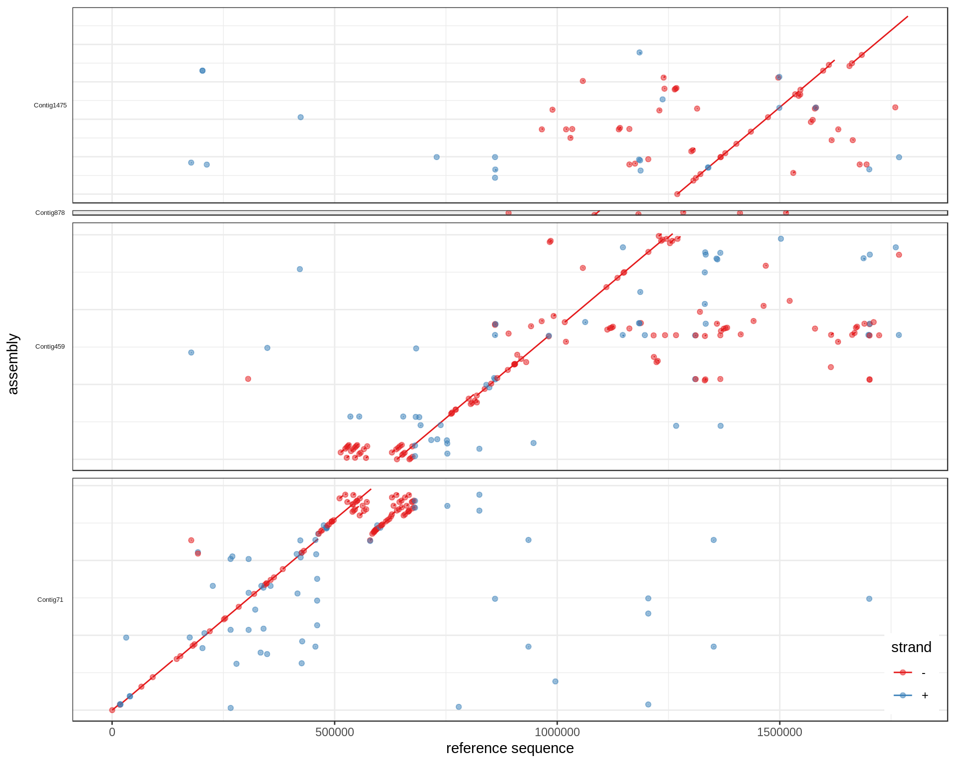
What we were aiming at:
Pretty good.
To also represent multiple reference regions in separate facets, change the facet_grid commands. Here we have only one reference region but the command would be:
ggplot(mumgp.filt.diag, aes(x=rs, xend=re, y=qs, yend=qe, colour=strand)) +
    geom_segment() + geom_point(alpha=.5) + theme_bw() +
    facet_grid(qid~rid, scales='free', space='free', switch='y') +
    theme(strip.text.y=element_text(angle=180, size=5), strip.background=element_blank(),
          legend.position=c(.99,.01), legend.justification=c(1,0),
          axis.text.y=element_blank(), axis.ticks.y=element_blank()) +
    xlab('reference sequence') + ylab('assembly') + scale_colour_brewer(palette='Set1')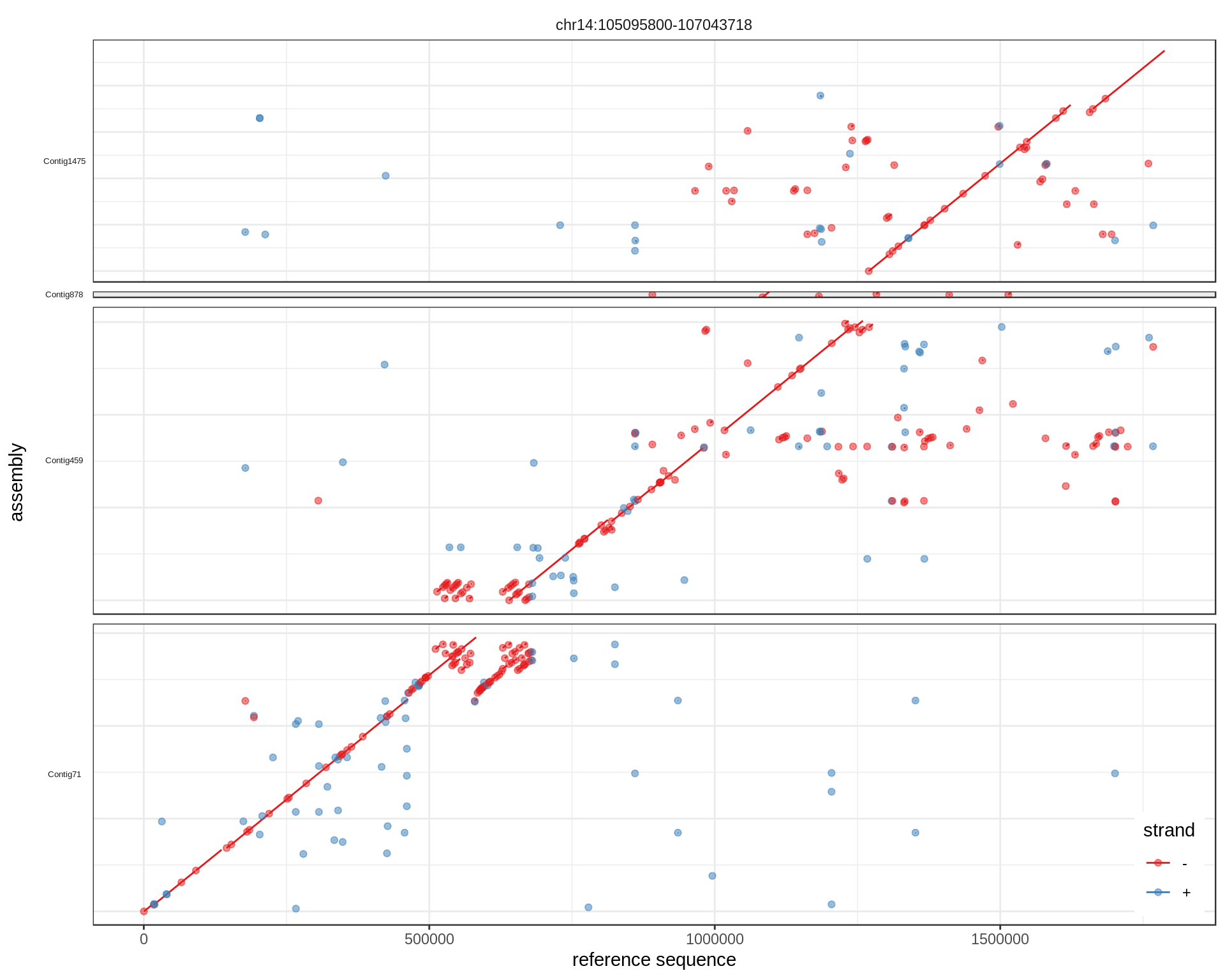
See also this GitHub issue.
Percent identity and coverage
Another useful MUMmerplot represents the position of each aligned segment and its percent similarity.
This graph could be useful to decide which size/similarity threshold to use when filtering low alignments.
mumgp %<>% mutate(similarity=1-error/abs(qe-qs))
mumgp.filt %<>% mutate(similarity=1-error/abs(qe-qs))

ggplot(mumgp, aes(x=rs, xend=re, y=similarity, yend=similarity)) + geom_segment() +
    theme_bw() + xlab('reference sequence') + ylab('similarity') + ggtitle('All contigs') +
    ylim(0,1)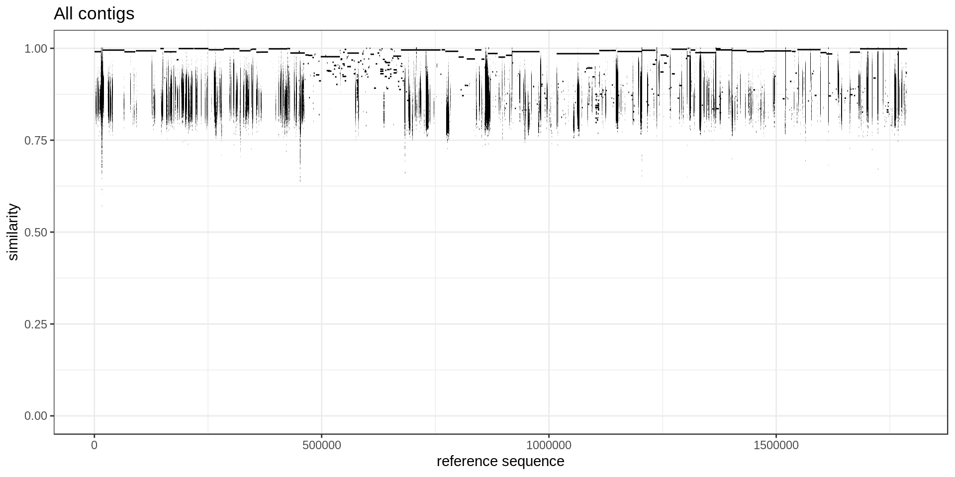
ggplot(mumgp.filt, aes(x=rs, xend=re, y=similarity, yend=similarity)) + geom_segment() +
    theme_bw() + xlab('reference sequence') + ylab('similarity') +
    ggtitle('At least 10 Kbp aligned') + ylim(0,1)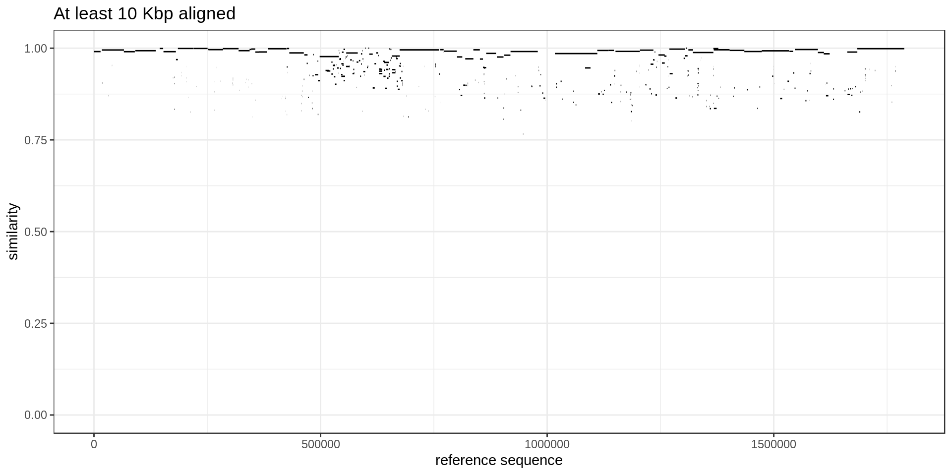
To better highlighted which region in the reference is covered, I annotate each base of the reference with the maximum similarity.
maxSimilarityDisjoin <- function(df){
  ref.ir = GRanges('X', IRanges(df$rs, df$re), similarity=df$similarity)
  ## Efficient clean up of low similarity within high similarity
  step = 1
  while(step>0){
    largealign = ref.ir[head(order(rank(-ref.ir$similarity), rank(-width(ref.ir))),step*1000)]
    ol = findOverlaps(ref.ir, largealign, type='within') %>% as.data.frame %>%
        mutate(simW=ref.ir$similarity[queryHits],
               simL=largealign$similarity[subjectHits]) %>% filter(simW<simL)
    if(length(largealign) == length(ref.ir)){
      step = 0
    } else {
      step = step + 1
    }
    ref.ir = ref.ir[-ol$queryHits]
  }
  ## Disjoin and annotate with the max similarity
  ref.dj = disjoin(c(ref.ir, GRanges('X', IRanges(min(df$rs), max(df$rs)), similarity=0)))
  ol = findOverlaps(ref.ir, ref.dj) %>% as.data.frame %>%
      mutate(similarity=ref.ir$similarity[queryHits]) %>%
      group_by(subjectHits) %>% summarize(similarity=max(similarity))
  ref.dj$similarity = 0
  ref.dj$similarity[ol$subjectHits] = ol$similarity
  as.data.frame(ref.dj)
}

mumgp.sim = maxSimilarityDisjoin(mumgp)

mumgp.sim %>% select(similarity, start, end) %>% gather(end, pos, 2:3) %>%
    ggplot() + geom_line(aes(x=pos, y=similarity), alpha=.5, color='red') + theme_bw() +
    xlab('reference sequence') + ylab('similarity') + ggtitle('All contigs') + ylim(0,1) +
    geom_segment(aes(x=rs, xend=re, y=similarity, yend=similarity), data=mumgp)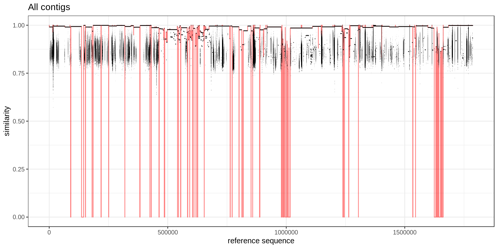
ggplot(mumgp.sim) + geom_segment(aes(x=start, xend=end, yend=similarity, y=similarity),
                                 color='red', size=2) +
    theme_bw() + xlab('reference sequence') + ylab('similarity') + ylim(0,1) +
    geom_segment(aes(x=rs, xend=re, y=similarity, yend=similarity), data=mumgp)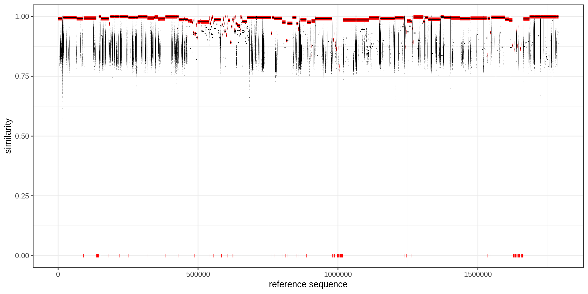
With this graph we could compare different assemblies or before/after filtering:
mumgp.filt.sim = maxSimilarityDisjoin(mumgp.filt)

mumgp.filt.m = rbind(mumgp.sim %>% mutate(filter='before'),
                     mumgp.filt.sim %>% mutate(filter='after'))

mumgp.filt.m %>% select(similarity, start, end, filter) %>% gather(end, pos, 2:3) %>%
    ggplot(aes(x=pos, y=similarity, colour=filter)) + geom_line(alpha=.8) + theme_bw() +
    xlab('reference sequence') + ylab('similarity') + ylim(0,1) +
    scale_colour_brewer(palette='Set1')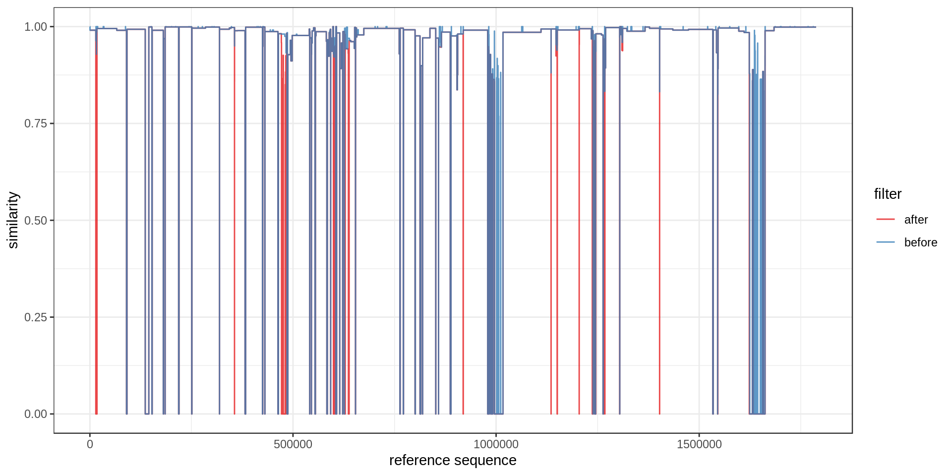
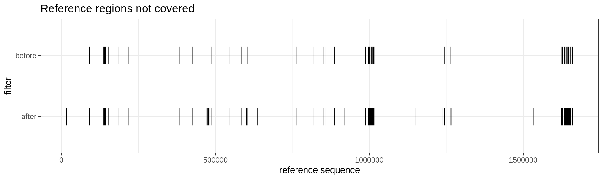
Not so pretty but we see that a few region are not covered any more after our filtering. Maybe something like this instead :
mumgp.filt.m %>% filter(similarity==0) %>%
    ggplot(aes(x=start, xend=end, y=filter, yend=filter)) + geom_segment(size=10) +
    theme_bw() + xlab('reference sequence') + ylab('filter') +
    scale_colour_brewer(palette='Set1') + ggtitle('Reference regions not covered')