 David Heller1,2,☯, Jean Monlong1,☯, Jonas Andreas Sibbesen1, Jouni Siren1, Jordan Eizenga1, Eric T. Dawson3,4, Erik Garrison1, Adam Novak1, Benedict Paten1,†
This manuscript (permalink) was automatically generated from jmonlong/manu-vgsv@a6adb10 on September 13, 2019.
Glenn Hickey1,☯, David Heller1,2,☯, Jean Monlong1,☯, Jonas Andreas Sibbesen1, Jouni Siren1, Jordan Eizenga1, Eric T. Dawson3,4, Erik Garrison1, Adam Novak1, Benedict Paten1,†
☯ — These authors contributed equally to this work
† — To whom correspondence should be addressed: bpaten@ucsc.edu
Structural variants (SVs) are significant components of genetic diversity and have been associated with diseases, but the technological challenges surrounding their representation and identification make them difficult to study relative to point mutations. Still, thousands of SVs have been characterized, and catalogs continue to improve with new technologies. In parallel, variation graphs have been proposed to represent human pangenomes, offering reduced reference bias and better mapping accuracy than linear reference genomes. We contend that variation graphs provide an effective means for leveraging SV catalogs for short-read SV genotyping experiments. In this work, we extend vg (a software toolkit for working with variation graphs) to support SV genotyping. We show that it is capable of genotyping insertions, deletions and inversions, even in the presence of small errors in the location of the SVs breakpoints. We then benchmark vg against state-of-the-art SV genotypers using three high-quality sequence-resolved SV catalogs generated by recent studies ranging up to 97,368 variants in size. We find that vg systematically produces the best genotype predictions in all datasets. In addition, we use assemblies from 12 yeast strains to show that graphs constructed directly from aligned de novo assemblies can improve genotyping compared to graphs built from intermediate SV catalogs in the VCF format. Our results demonstrate the power of variation graphs for SV genotyping. Beyond single nucleotide variants and short insertions/deletions, the vg toolkit now incorporates SVs in its unified variant calling framework and provides a natural solution to integrate high-quality SV catalogs and assemblies.
A structural variant (SV) is a genomic mutation involving 50 or more base pairs. SVs can take several forms such as deletions, insertions, inversions, translocations or other complex events.
Due to their greater size, SVs often have a larger impact on phenotype than smaller events such as single nucleotide variants (SNVs) and small insertions and deletions (indels)[1]. Indeed, SVs have long been associated with developmental disorders, cancer and other complex diseases and phenotypes[2].
Despite their importance, SVs remain much more poorly studied than their smaller mutational counterparts. This discrepancy stems from technological limitations. Short read sequencing has provided the basis of most modern genome sequencing studies due to its high base-level accuracy and relatively low cost, however, it is poorly suited for discovering SVs. The central obstacle is in mapping short reads to the human reference genome. It is generally difficult or impossible to unambiguously map a short read if the sample whose genome is being analyzed differs substantially from the reference at the read’s location. The large size of SVs virtually guarantees that short reads derived from them will not map to the linear reference genome. For example, if a read corresponds to sequence in the middle of a large reference-relative insertion, then there is no location in the reference that corresponds to a correct mapping. The best result a read mapper could hope to produce would be to leave it unmapped. Moreover, SVs often lie in repeat-rich regions, which further frustrate read mapping algorithms.
Short reads can be more effectively used to genotype known SVs. This is important, as even though efforts to catalog SVs with other technologies have been highly successful, their cost currently prohibits their use in large-scale studies that require hundreds or thousands of samples such as disease association studies. Traditional SV genotypers start from reads that were mapped to a reference genome, extracting aberrant mapping that might support the presence of the SV of interest. State-of-art methods like SVTyper[3] and Delly[4] typically focus on split reads and paired reads mapped too close or too far from each other. These discordant reads are tallied and remapped to the reference sequence modified with the SV of interest in order to genotype deletions, insertions, duplications, inversions and translocations. SMRT-SV v2 uses a different approach: the reference genome is augmented with SV-containing sequences as alternate contigs and the resulting mappings are evaluated with a machine learning model trained for this purpose[5].
The catalog of known SVs in human is quickly expanding. Several large-scale projects have used short-read sequencing and extensive discovery pipelines on large cohorts, compiling catalogs with tens of thousands of SVs in humans[6,7], using split read and discordant pair based methods like SVTyper[3] and Delly[4] to find SVs using short read sequencing. More recent studies using long-read or linked-read sequencing have produced large catalogs of structural variation, the majority of which was novel and sequence-resolved[10,11,5,8,9]. These technologies are also enabling the production of high-quality de novo genome assemblies[12,8], and large blocks of haplotype-resolved sequences[13]. Such technical advances promise to expand the amount of known genomic variation in humans in the near future, and further power SV genotyping studies. Representing known structural variation in the wake of increasingly larger datasets poses a considerable challenge, however. VCF, the standard format for representing small variants, is unwieldy when used for SVs due its unsuitability for expressing nested or complex variants. Another strategy consists in incorporating SVs into a linear pangenome reference via alt contigs, but it also has serious drawbacks. Alt contigs tend to increase mapping ambiguity. In addition, it is unclear how to scale this approach as SV catalogs grow.
Pangenomic graph reference representations offer an attractive approach for storing genetic variation of all types[14]. These graphical data structures can seamlessly represent both SVs and point mutations using the same semantics. Moreover, including known variants in the reference makes both read mapping and variant calling variant-aware. This leads to benefits in terms of accuracy and sensitivity[15,16,17]. The coherency of this model allows different variant types to be called and scored simultaneously in a unified framework.
vg is the first openly available variation graph tool to scale to multi-gigabase genomes. It provides read mapping, variant calling and visualization tools[15]. In addition, vg can build graphs both from variant catalogs in the VCF format and from assembly alignments.
Other tools have used genome graphs or pangenomes to genotype variants. GraphTyper realigns mapped reads to a graph built from known SNVs and short indels using a sliding-window approach[18]. BayesTyper first builds a set of graphs from known variants including SVs, then genotypes variants by comparing the distribution of k-mers in the sequencing reads with the k-mers of haplotype candidate paths in the graph[19]. SMRT-SV v2 uses a different approach: the reference genome is augmented with SV-containing sequences as alternate contigs and the resulting mappings are evaluated with a machine learning model trained for this purpose[5]. These graph-based approaches showed clear advantages over standard methods that use only the linear reference.
In this work, we present a SV genotyping framework based on the variation graph model and implemented in the vg toolkit. We show that this method is capable of genotyping known deletions, insertions and inversions, and that its performance is not inhibited by small errors in the specification of SV allele breakpoints. We evaluated the genotyping accuracy of our approach using simulated and real Illumina reads and a pangenome built from SVs discovered in recent long-read sequencing studies[20,21,22,5], We also compared vg’s performance with state-of-the-art SV genotypers: SVTyper[3], Delly[4], BayesTyper[19] and SMRT-SV v2[5]. Across these three datasets that we tested, which range in size from 26k to 97k SVs, vg is the best performing SV genotyper on real short-read data for all SV types. Finally, we demonstrate that a pangenome graph built from the alignment of de novo assemblies of diverse Saccharomyces cerevisiae strains improves SV genotyping performance.
We used vg to implement a straightforward SV genotyping pipeline. Reads are mapped to the graph and used to compute the read support for each node and edge (see Supplementary Information for a description of the graph formalism). Sites of variation are then identified using the snarl (aka “bubble”) decomposition as described in [23], each resulting site being represented as a subgraph of the larger graph. For each site, we determine the two most supported paths (haplotypes), and use their relative support in the read evidence to produce a genotype at that site (Figure 1a). We describe the pipeline in more detail in Methods. We rigorously evaluated the accuracy of our method on a variety of datasets, and present these results in the remainder of this section.
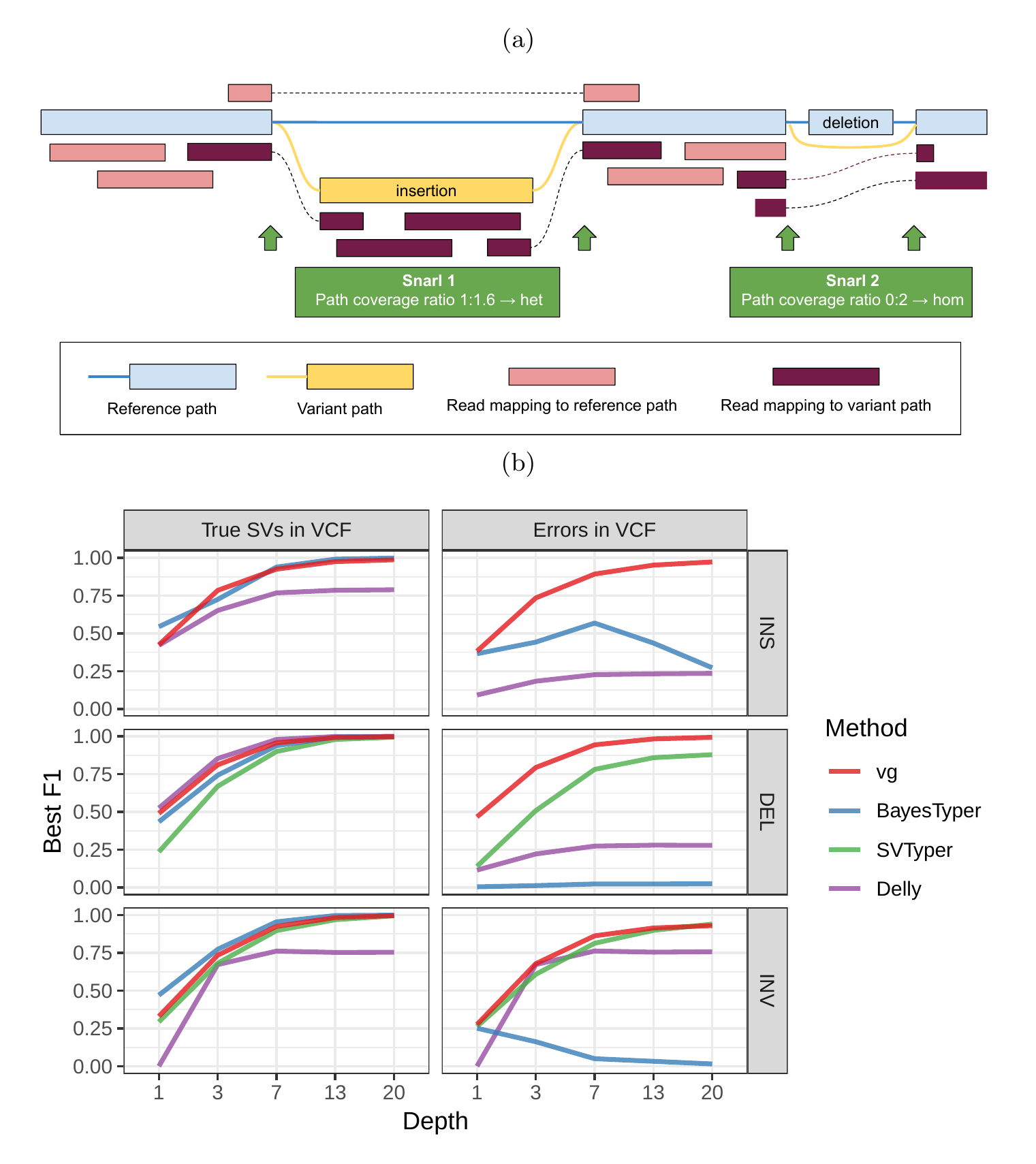
As a proof of concept, we simulated genomes and different types of SVs with a size distribution matching real SVs[20]. We compared vg against SVTyper, Delly, and BayesTyper across different levels of sequencing depth. We also added some errors (1-10bp) to the location of the breakpoints to investigate their effect on genotyping accuracy (see Methods). The results are shown in Figure 1b.
When using the correct breakpoints, vg tied with Delly as the best genotyper for deletions, and with BayesTyper as the best genotyper for insertions. For inversions, vg was the second best genotyper after BayesTyper. The differences between the methods were the most visible at lower sequencing depth. In the presence of 1-10 bp errors in the breakpoint locations, the performance of Delly and BayesTyper dropped significantly (Figure 1b). The dramatic drop for BayesTyper can be explained by its k-mer-based approach that requires precise breakpoints. In contrast, vg was only slightly affected by the presence of errors. For vg, the F1 scores for all SV types decreased no more than 0.07. Overall, these results show that vg is capable of genotyping SVs and is robust to breakpoint inaccuracies in the input VCF.
72,485 structural variants from The Human Genome Structural Variation Consortium (HGSVC) were used to benchmark the genotyping performance of vg against the three other SV genotyping methods. This high-quality SV catalog was generated from three samples using a consensus from different sequencing, phasing, and variant calling technologies[20]. The three individual samples represent different human populations: Han Chinese (HG00514), Puerto-Rican (HG00733), and Yoruban Nigerian (NA19240). We used these SVs to construct a graph with vg and as input for the other genotypers. Using short sequencing reads, the SVs were genotyped and compared with the genotypes in the original catalog (see Methods).
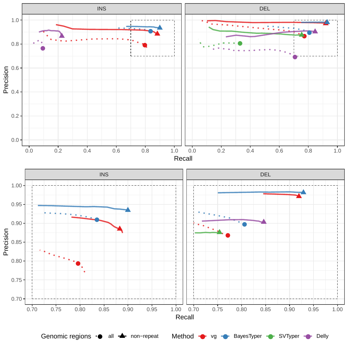
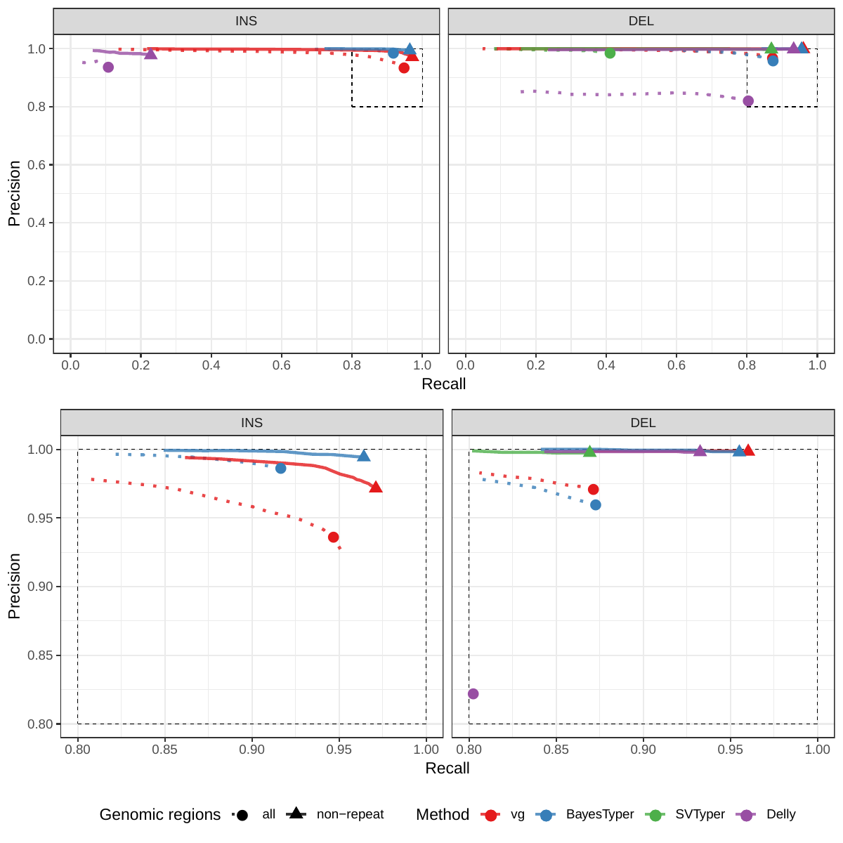
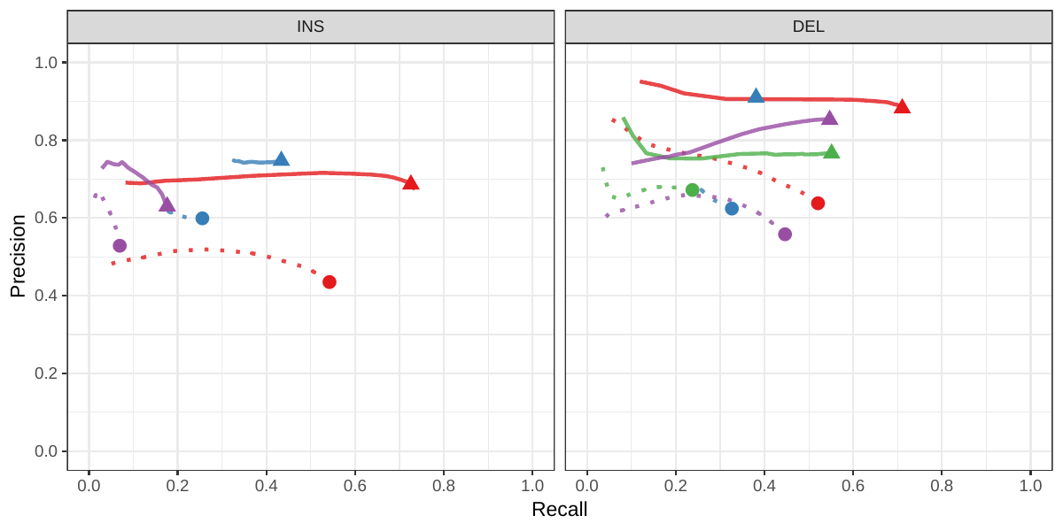
First we compared the methods using simulated reads for HG00514. This represents the ideal situation where the SV catalog exactly matches the SVs supported by the reads. While vg outperformed Delly and SVTyper, BayesTyper showed the best F1 score and precision-recall trade-off (Figures 2a and S1, Table S1). When restricting the comparisons to regions not identified as tandem repeats or segmental duplications, the genotyping predictions were significantly better for all methods, with vg almost as good as BayesTyper on deletions (F1 of 0.944 vs 0.955). We observed similar results when evaluating the presence of an SV call instead of the exact genotype (Figures 2a and S2). Overall, both graph-based methods, vg and BayesTyper, outperformed the other two methods tested.
![Figure 2: Structural variants from the HGSVC and Genome in a Bottle datasets. HGSVC: Simulated and real reads were used to genotype SVs and compared with the high-quality calls from Chaisson et al.[20]. Reads were simulated from the HG00514 individual. Using real reads, the three HG00514, HG00733, and NA19240 individuals were tested. GIAB: Real reads from the HG002 individual were used to genotype SVs and compared with the high-quality calls from the Genome in a Bottle consortium[21,22,24]. a) Maximum F1 score for each method (color), across the whole genome or focusing on non-repeat regions (x-axis). We evaluated the ability to predict the presence of an SV (transparent bars) and the exact genotype (solid bars). Results are separated across panels by variant type: insertions and deletions. SVTyper cannot genotype insertions, hence the missing bars in the top panels. b) Maximum F1 score for different size classes when evaluating on the presence of SVs across the whole genome. c) Size distribution of SVs in the HGSVC and GIAB catalogs.](images/panel2.png)
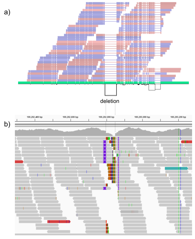
We then repeated the analysis using real Illumina reads from the three HGSVC samples to benchmark the methods on a more realistic experiment. Here, vg clearly outperformed other approaches (Figures 2a and S3). In non-repeat regions and across the whole genome, the F1 scores and precision-recall AUC were higher for vg compared to other methods. For example, for deletions in non-repeat regions, the F1 score for vg was 0.801 while the second best method, Delly, had a F1 score of 0.692. We observed similar results when evaluating the presence of an SV call instead of the exact genotype (Figures 2a and S4). In addition, vg’s performance was stable across the spectrum of SV sizes (Figure 2b-c). Figure 3 shows an example of an exonic deletion that was correctly genotyped by vg but not by the other methods.
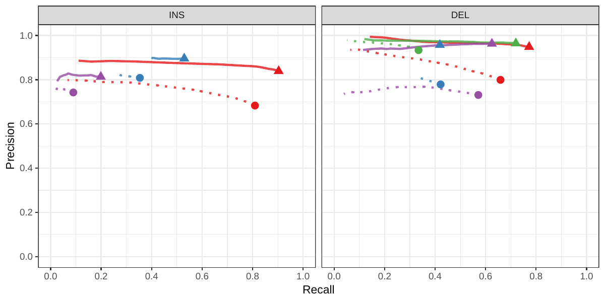
The Genome in a Bottle (GiaB) consortium is currently producing a high-quality SV catalog for an Ashkenazim individual (HG002)[21,22,24]. Dozens of SV callers operating on datasets from short, long, and linked reads were used to produce this set of SVs. We evaluated the SV genotyping methods on this sample as well using the GIAB VCF, which also contains parental calls (HG003 and HG004), all totalling 30,224 SVs. vg performed similarly on this dataset as on the HGSVC dataset, with a F1 score of 0.75 for both insertions and deletions in non-repeat regions (Figures 2, S5 and S6, and Table S2). As before, other methods produced lower F1 scores in most cases, although Delly and BayesTyper predicted better genotypes for deletions in non-repeat regions.
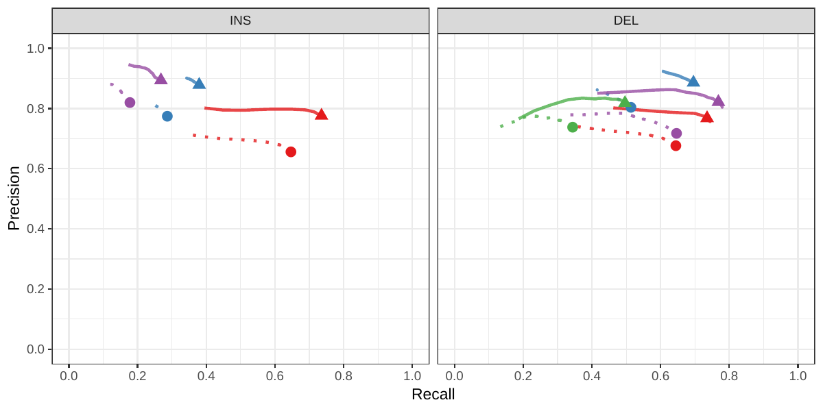
A recent study by Audano et al. generated a catalog of 97,368 SVs (referred as SVPOP below) using long-read sequencing across 15 individuals[5]. These variants were then genotyped from short reads across 440 individuals using the SMRT-SV v2 genotyper, a machine learning-based tool implemented for that study. The SMRT-SV v2 genotyper was trained on a pseudo-diploid genome constructed from high quality assemblies of two haploid cell lines (CHM1 and CHM13) and a single negative control (NA19240). We first used vg to genotype the SVs in this two-sample training dataset using 30X coverage reads, and compared the results with the SMRT-SV v2 genotyper. vg was systematically better at predicting the presence of an SV for both SV types, but SMRT-SV v2 produced better genotypes for deletions (see Figures 4, S7 and S8, and Table S3). To compare vg and SMRT-SV v2, we then genotyped SVs from the entire SVPOP catalog with both methods, using the read data from the three HGSVC samples described above. Given that the the SVPOP catalog contains these three samples, we once again evaluated accuracy by using the long-read genotypes as a baseline of comparison.
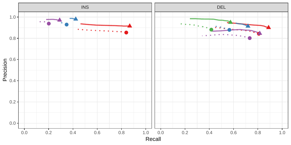
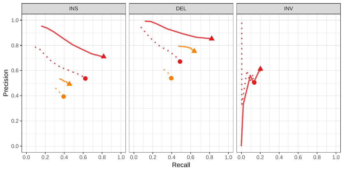
Compared to SMRT-SV v2, vg had a better precision-recall curve and a higher F1 for both insertions and deletions (SVPOP in Figures 4 and S9, and Table S4). Of note, SMRT-SV v2 produces no-calls in regions where the read coverage is too low, and we observed that its recall increased when filtering these regions out the input set. Interestingly, vg performed well even in regions where SMRT-SV v2 produced no-calls (Figure S10 and Table S5). Audano et al. discovered 217 sequence-resolved inversions using long reads, which we attempted to genotype. vg correctly predicted the presence of around 14% of the inversions present in the three samples (Table S4). Inversions are often complex, harboring additional variation that makes their characterization and genotyping challenging.
![Figure 4: Structural variants from SMRT-SV v2 [5]. The pseudo-diploid genome built from two CHM cell lines and one negative control sample was originally used to train SMRT-SV v2 in Audano et al.[5]. It contains 16,180 SVs. The SVPOP panel shows the combined results for the HG00514, HG00733, and NA19240 individuals, three of the 15 individuals used to generate the high-quality SV catalog in Audano et al. [5]. Here, we report the maximum F1 score (y-axis) for each method (color), across the whole genome or focusing on non-repeat regions (x-axis). We evaluated the ability to predict the presence of an SV (transparent bars) and the exact genotype (solid bars). Genotype information is not available in the SVPOP catalog hence genotyping performance could not be evaluated.](images/chmpd-svpop-best-f1.png)
We can construct variation graphs directly from whole genome alignments of multiple de novo assemblies[15]. This bypasses the need for generating an explicit variant catalog relative to a linear reference, which could be a source of error due to the reference bias inherent in read mapping and variant calling. Genome alignments from graph-based software such as Cactus [25] can contain complex structural variation that is extremely difficult to represent, let alone call, outside of a graph, but which is nevertheless representative of the actual genomic variation between the aligned assemblies. We sought to establish if graphs built in this fashion provide advantages for SV genotyping.
To do so, we analyzed public sequencing datasets for 12 yeast strains from two related clades (S. cerevisiae and S. paradoxus) [26]. We distinguished two different strain sets, in order to assess how the completeness of the graph affects the results. For the all strains set, all 12 strains were used, with S.c. S288C as the reference strain. For the five strains set, S.c. S288C was used as the reference strain, and we selected two other strains from each of the two clades (see Methods). We compared genotyping results from two different types of genome graphs. The first graph (VCF graph) was created from the linear reference genome of the S.c. S288C strain and a set of SVs relative to this reference strain in VCF format identified from the other assemblies in the respective strain set by three methods: Assemblytics [27], AsmVar [28] and paftools [29]. The second graph (cactus graph) was derived from a multiple genome alignment of the strains in the respective strain set using Cactus [25]. The VCF graph is mostly linear and highly dependent on the reference genome. In contrast, the cactus graph is structurally complex and relatively free of reference bias.
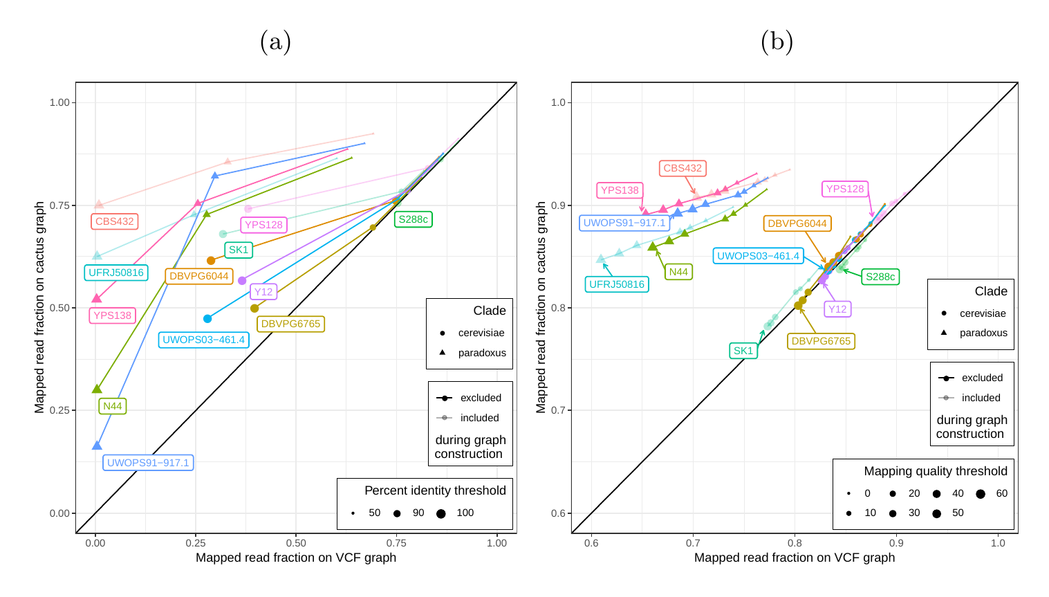
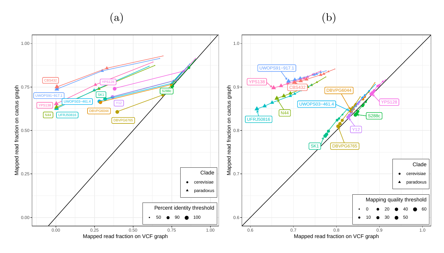
First, we tested our hypothesis that the cactus graph has higher mappability due to its better representation of sequence diversity among the yeast strains (see Supplementary Information). Generally, more reads mapped to the cactus graph with high identity (Figures S12a and S13a) and high mapping quality (Figures S12b and S13b) than to the VCF graph.
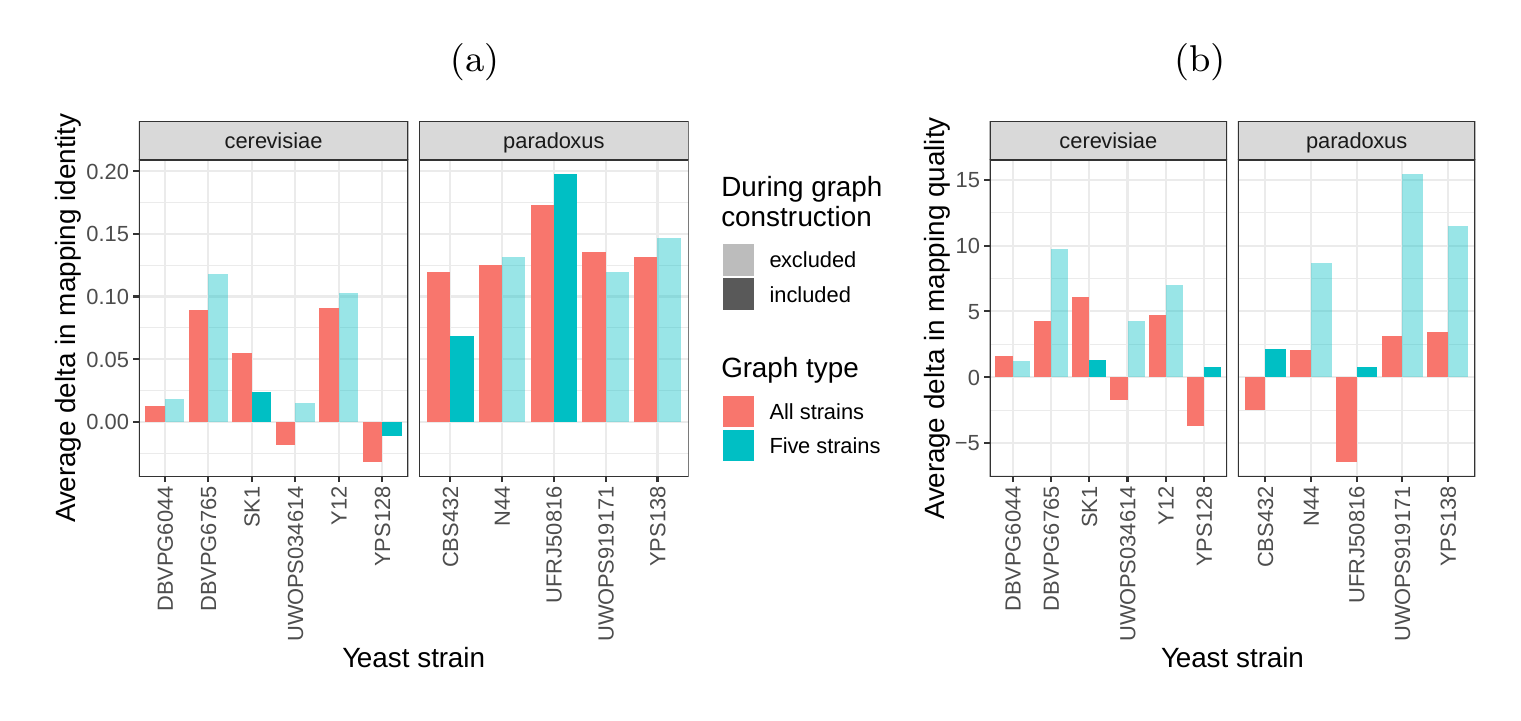
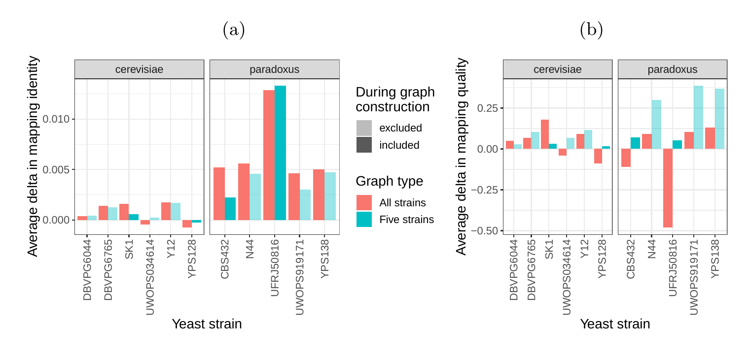
Next, we compared the SV genotyping performance of both graph types. We mapped short reads from the 11 non-reference strains to both graphs and called variants for each strain using the vg toolkit’s variant calling module (see Methods). There is no gold standard call set for these samples, so we used an indirect measure of SV calling accuracy. We evaluated each SV call set based on the alignment of reads to a sample graph constructed from the call set (see Methods). If a given call set is correct, we expect that reads from the same sample will be mapped with high identity and confidence to the corresponding sample graph. To specifically quantify mappability in SV regions we excluded reads that produced identical mapping quality and identity on both sample graphs and an empty sample graph containing the linear reference only (see Methods and Figure S14 for results from all reads). Then, we analyzed the average delta in mapping identity and mapping quality of the remaining short reads between both sample graphs (Figures 5a and b).
For most of the strains, we observed an improvement in mapping identity of the short reads on the cactus sample graph compared to the VCF sample graph. The mean improvement in mapping identity across the strains was 8.0% and 8.5% for the all strains set graphs and the five strains set graphs, respectively. Generally, the improvement in mapping identity was larger for strains in the S. paradoxus clade (mean of 13.7% and 13.3% for the two strain sets, respectively) than for strains in the S. cerevisiae clade (mean of 3.3% and 4.4%). While the higher mapping identity indicated that the cactus graph represents the reads better (Figure 5a), the higher mapping quality confirmed that this did not come at the cost of added ambiguity or a more complex graph (Figure 5b). For most strains, we observed an improvement in mapping quality of the short reads on the cactus sample graph compared to the VCF sample graph (mean improvement across the strains of 1.0 and 5.7 for the two strain sets, respectively).
Overall, vg was the most accurate SV genotyper in our benchmarks. These results show that variant calling benefits from variant-aware read mapping and graph based genotyping, a finding consistent with previous studies[15,16,17,18,19]. We took advantage of newly released datasets for our evaluation, which feature up to 3.7 times more variants than the more widely-used GIAB benchmark. More and more large-scale projects are using low cost short-read technologies to sequence the genomes of thousands to hundreds of thousands of individuals (e.g. the Pancancer Analysis of Whole Genomes[30], the Genomics England initiative[31], and the TOPMed consortium[32]). We believe pangenome graph-based approaches will improve both how efficiently SVs can be represented, and how accurately they can be genotyped with this type of data.
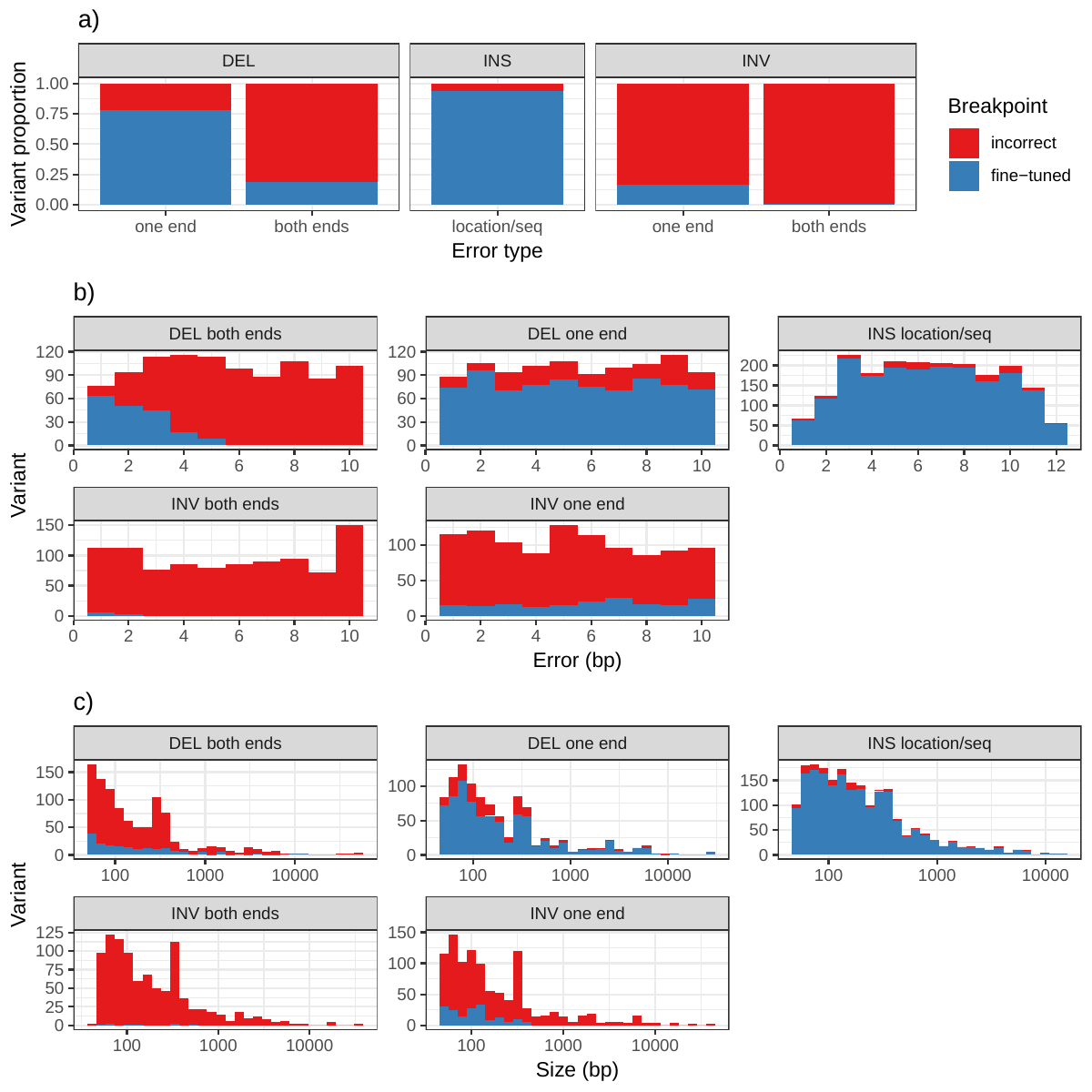
A particular advantage of our method is that it does not require exact breakpoint resolution in the variant library. Our simulations showed that vg’s SV genotyping algorithm is robust to errors of as much as 10 bp in breakpoint location. However, there is an upper limit to this flexibility, and we find that vg cannot accurately genotype variants with much higher uncertainty in the breakpoint location (like those discovered through read coverage analysis). vg is also capable of fine-tuning SV breakpoints by augmenting the graph with differences observed in read alignments. Simulations showed that this approach can usually correct small errors in SV breakpoints (Figure S11 and Table S6).
vg uses a unified framework to call and score different variant types simultaneously. In this work, we only considered graphs containing certain types of SVs, but the same methods can be extended to a broader range of graphs. For example, we are interested in evaluating how genotyping SVs together with SNPs and small indels using a combined graph effects the accuracy of studying either alone. The same methods used for genotyping known variants in this work can also be extended to call novel variants by first augmenting the graph with edits from the mapped reads. This approach, which was used only in the breakpoint fine-tuning portion of this work, could be further used to study small variants around and nested within SVs. Novel SVs could be called by augmenting the graph with long-read mappings. vg is entirely open source, and its ongoing development is supported by a growing community of researchers and users with common interest in scalable, unbiased pangenomic analyses and representation. We expect this collaboration to continue to foster increases in the speed, accuracy and applicability of methods based on pangenome graphs in the years ahead.
Our results suggest that constructing a graph from de novo assembly alignment instead of a VCF leads to better SV genotyping. High quality de novo assemblies for human are becoming more and more common due to improvements in technologies like optimized mate-pair libraries[33] and long-read sequencing[12]. We expect future graphs to be built from the alignment of numerous de novo assemblies, and we are presently working on scaling our assembly-based pipeline to human-sized genome assemblies. Another challenge is creating genome graphs that integrate assemblies with variant-based data resources. One possible approach is to progressively align assembled contigs into variation graphs constructed from variant libraries, but methods for doing so are still experimental.
In this study, the vg toolkit was compared to existing SV genotypers across several high-quality SV catalogs. We showed that its method of mapping reads to a variation graph leads to better SV genotyping compared to other state of the art methods. This work introduces a flexible strategy to integrate the growing number of SVs being discovered with higher resolution technologies into a unified framework for genome inference. Our work on whole genome alignment graphs shows the benefit of directly utilizing de novo assemblies rather than variant catalogs to integrate SVs in genome graphs. We expect this latter approach to increase in significance as the reduction in long read sequencing costs drives the creation of numerous new de novo assemblies. We envision a future in which the lines between variant calling, alignment, and assembly are blurred by rapid changes in sequencing technology. Fully graph based approaches, like the one we present here, will be of great utility in this new phase of genome inference.
In vg call, we implemented a simple variant caller capable of operating on any kind of variation that can be represented in variation graphs. The algorithm uses a genome graph as a structuring prior, and consumes read mappings to the graph to drive the inference of the true genomic state at each locus. Here, we apply vg call to genotype structural variants already present in the graph, but the same algorithm can also be used for smaller variants such as SNPs, as well as making de-novo calls. The algorithm, illustrated in Figure 1a, proceeds through three main phases:
toil-vg is a set of Python scripts for simplifying vg tasks such as graph construction, read mapping and SV genotyping. It uses the Toil workflow engine [34] to seamlessly run pipelines locally, on clusters, or on the cloud. All variation graph analyses in this report used toil-vg, with the exact commands available at github.com/vgteam/sv-genotyping-paper. The principal toil-vg commands used are described below.
toil-vg construct automates graph construction and indexing following the best practices put forth by the vg community. It parallelizes graph construction across different sequences from the reference FASTA, and creates different whole-genome indexes side by side when possible. When available, toil-vg construct can use phasing information from the input VCF to preserve haplotypes in the GCSA2 pruning step, as well as to extract haploid sequences to simulate from.
toil-vg map splits the input reads into batches, maps each batch in parallel, and merges the result.
Due to the high memory requirements of the current implementation of vg call, toil-vg call splits the input graph into 2.5Mb overlapping chunks along the reference path. Each chunk is called independently in parallel and the results are concatenated into the output VCF.
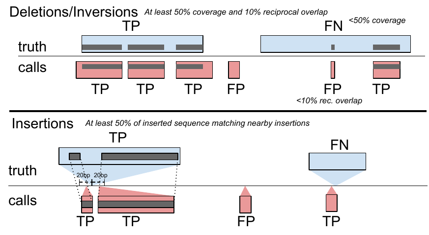
toil-vg sveval evaluates the SV calls relative to a truth set. The variants are first normalized with bcftools norm (1.9) to ensure consistent representation between called variants and baseline variants[35]. We then implemented an overlap-based strategy to compare SVs and compute evaluation metrics (sveval R package: https://github.com/jmonlong/sveval). Figure S15 shows an overview of the SV evaluation approach which is described below.
For deletions and inversions, we begin by computing the overlaps between the SVs in the call set and the truth set. For each variant we then compute the proportion of its region that is covered by a variant in the other set, considering only variants overlapping with at least 10% reciprocal overlap. If this coverage proportion is higher than 50%, we consider the variant covered. True positives (TPs) are covered variants from the call set (when computing the precision) or the truth set (when computing the recall). Variants from the call set are considered false positives (FPs) if they are not covered by the truth set. Conversely, variants from the truth set are considered false negatives (FNs) if they are not covered by the call set.
For insertions, we select pairs of insertions that are located no farther than 20 bp from each other. We then align the inserted sequences using a Smith-Waterman alignment. For each insertion we compute the proportion of its inserted sequence that aligns a matched variant in the other set. If this proportion is at least 50% the insertions are considered covered. Covering relationships are used to define TPs, FPs, and FNs the same way as for deletions and inversions.
The coverage statistics are computed using any variant larger than 1 bp but a minimum size is required for a variant to be counted as TP, FP, or FN. In this work, we used the default minimum SV size of 50 bp.
sveval accepts VCF files with symbolic or explicit representation of the SVs. If the explicit representation is used, multi-allelic variants are split and their sequences right-trimmed. When using the explicit representation and when the REF and ALT sequences are longer than 10 bp, the reverse-complement of the ALT sequence is aligned to the REF sequence to identify potential inversions. If more than 80% of the sequence aligns, it is classified as an inversion.
We assess both the ability to predict the presence of an SV as well as the full genotype. For the presence evaluation, both heterozygous and homozygous alternate SVs are compared jointly using the approach described above. To compute genotype-level metrics, the heterozygous and homozygous SVs are compared separately. Before splitting the variants by genotype, pairs of heterozygous variants with reciprocal overlap of at least 80% are merged into a homozygous ALT variant. To handle fragmented variants, consecutive heterozygous variants located at less that 20 bp from each other are first merged into larger heterozygous variants.
Precision-recall curves are produced by successively filtering out variants of low-quality. By default the QUAL field in the VCF file is used as the quality information. If QUAL is missing (or contains only 0s), the genotype quality in the GQ field is used.
The evaluation is performed using all variants or using only variants within high-confidence regions. In most analysis, the high-confidence regions are constructed by excluding segmental duplications and tandem repeats (using the respective tracks from the UCSC Genome Browser). For the GIAB analysis, we used the Tier 1 high-confidence regions provided by the GIAB consortium in version 0.6.
Where not specified otherwise BayesTyper was run as follows. Raw reads were mapped to the reference genome using bwa mem (citation: https://arxiv.org/abs/1303.3997) (0.7.17). GATK haplotypecaller[36] (3.8) and Platypus[37] (0.8.1.1) with assembly enabled were run on the mapped reads to call SNVs and short indels (<50bp) needed by BayesTyper for correct genotyping. The VCFs with these variants were then normalised using bcftools norm (1.9) and combined with the SVs across samples using bayesTyperTools combine to produce the input candidate set. k-mers in the raw reads were counted using kmc (citation: https://academic.oup.com/bioinformatics/article/33/17/2759/3796399) (3.1.1) with a k-mer size of 55. A Bloom filter was constructed from these k-mers using bayesTyperTools makeBloom. Finally, variants were clustered and genotyped using bayestyper cluster and bayestyper genotype, respectively, with default parameters except --min-genotype-posterior 0. Non-PASS variants and non-SVs (GATK and Platypus origin) were filtered prior to evaluation using bcftools filter and filterAlleleCallsetOrigin, respectively.
The delly call command was run on the reads mapped by bwa mem, the reference genome FASTA file, and the VCF containing the SVs to genotype (converted to their explicit representations).
The VCF containing deletions was converted to symbolic representation and passed to svtyper with the reads mapped by bwa mem. The output VCF was converted back to explicit representation using bayesTyperTools convertAllele to facilitate variant normalization before evaluation.
SMRT-SV v2 was run with the “30x-4” model and min-call-depth 8 cutoff. It was run only on VCFs created by SMRT-SV, for which the required contig BAMs were available. The Illumina BAMs used where the same as the other methods described above. The output VCF was converted back to explicit representation to facilitate variant normalization later.
We simulated a synthetic genome with 1000 insertions, deletions and inversions. We separated each variant from the next by a buffer of at least 500 bp. The sizes of deletions and insertions followed the distribution of SV sizes from the HGSVC catalog. We used the same size distribution as deletions for inversions. A VCF file was produced for three simulated samples with genotypes chosen uniformly between homozygous reference, heterozygous, and homozygous alternate.
We created another VCF file containing errors in the SV breakpoint locations. We shifted one or both breakpoints of deletions and inversions by distances between 1 and 10 bp. The locations and sequences of insertions were also modified, either shifting the variants or shortening them at the flanks, again by up to 10 bp.
Paired-end reads were simulated using vg sim on the graph that contained the true SVs. Different read depths were tested: 1x, 3x, 7x, 10x, 13x, 20x. The base qualities and sequencing errors were trained to resemble real Illumina reads from NA12878 provided by the Genome in a Bottle Consortium.
The genotypes called in each experiment (genotyping method/VCF with or without errors/sequencing depth) were compared to the true SV genotypes to compute the precision, recall and F1 score (see toil-vg sveval).
vg can call variants after augmenting the graph with the read alignments to discover new variants (see toil-vg call). We tested if this approach could fine-tune the breakpoint location of SVs in the graph. We started with the graph that contained approximate SVs (1-10 bp errors in breakpoint location) and 20x simulated reads from the simulation experiment (see Simulation experiment). The variants called after graph augmentation were compared with the true SVs. We considered fine-tuning correct if the breakpoints matched exactly.
We first obtained phased VCFs for the three Human Genome Structural Variation Consortium (HGSVC) samples from Chaisson et al.[20] and combined them with bcftools merge. A variation graph was created and indexed using the combined VCF and the HS38D1 reference with alt loci excluded. The phasing information was used to construct a GBWT index[38], from which the two haploid sequences from HG00514 were extracted as a graph. Illumina read pairs with 30x coverage were simulated from these sequences using vg sim, with an error model learned from real reads from the same sample. These simulated reads reflect an idealized situation where the breakpoints of the SVs being genotyped are exactly known a priori. The reads were mapped to the graph, and the mappings used to genotype the SVs in the graph. Finally, the SV calls were compared back to the HG00514 genotypes from the HGSVC VCF. We repeated the process with the same reads on the linear reference, using bwa mem for mapping and Delly, SVTyper and BayesTyper for SV genotyping.
We downloaded Illumina HiSeq 2500 paired end reads from the EBI’s ENA FTP site for the three samples, using Run Accessions ERR903030, ERR895347 and ERR894724 for HG00514, HG00733 and NA19240, respectively. We ran the graph and linear mapping and genotyping pipelines exactly as for the simulation, and aggregated the comparison results across the three samples. We used BayesTyper to jointly genotype the 3 samples.
We obtained version 0.5 of the Genome in a Bottle (GIAB) SV VCF for the Ashkenazim son (HG002) and his parents from the NCBI FTP site. We obtained Illumina reads as described in Garrison et al.[15] and downsampled them to 50x coverage. We used these reads as input for vg call and the other SV genotyping pipelines described above (though with GRCh37 instead of GRCh38). For BayesTyper, we created the input variant set by combining the GIAB SVs with SNV and indels from the same study. Variants with reference allele or without a determined genotype for HG002 in the GIAB call set (10,569 out of 30,224) were considered “false positives” as a proxy measure for precision. These variants correspond to putative technical artifacts and parental calls not present in HG002. For the evaluation in high confidence regions, we used the Tier 1 high-confidence regions provided by the GIAB consortium in version 0.6.
The SMRT-SV v2 genotyper can only be used to genotype sequence-resolved SVs present on contigs with known SV breakpoints, such as those created by SMRT-SV v2, and therefore could not be run on the simulated, HGSVC, or GIAB call sets. The authors shared their training and evaluation set: a pseudodiploid sample constructed from combining the haploid CHM1 and CHM13 samples (CHMPD), and a negative control (NA19240). The high quality of the CHM assemblies makes this set an attractive alternative to using simulated reads. We used this two-sample pseudodiploid VCF along with the 30X read set to construct, map and genotype with vg, and also ran SMRT-SV v2 genotyper with the “30x-4” model and min-call-depth 8 cutoff, and compared the two back to the original VCF.
In an effort to extend this comparison from the training data to a more realistic setting, we reran the three HGSVC samples against the SMRT-SV v2 discovery VCF (SVPOP, which contains 12 additional samples in addition to the three from HGSVC) published by Audano et al.[5] using vg and SMRT-SV v2 Genotyper. The discovery VCF does not contain genotypes. In consequence, we were unable to distinguish between heterozygous and homozygous genotypes, and instead considered only the presence or absence of a non-reference allele for each variant.
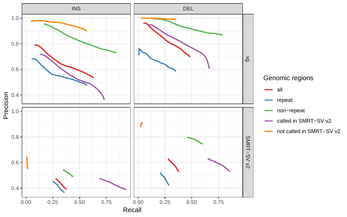
SMRT-SV v2 produces explicit no-call predictions when the read coverage is too low to produce accurate genotypes. These no-calls are considered homozygous reference in the main accuracy evaluation. We also explored the performance of vg and SMRT-SV v2 in different sets of regions (Figure S10 and Table S5):
For the analysis of graphs from de novo assemblies, we utilized publicly available PacBio-derived assemblies and Illumina short read sequencing datasets for 12 yeast strains from two related clades (Table 1) [26]. We constructed graphs from two different strain sets: For the five strains set, we selected five strains for graph contruction (S.c. SK1, S.c. YPS128, S.p. CBS432, S.p. UFRJ50816 and S.c. S288C). We randomly selected two strains from different subclades of each clade as well as the reference strain S.c. S288C. For the all strains set in contrast, we utilized all twelve strains for graph contruction. We constructed two different types of genome graphs from the PacBio-derived assemblies of the five or twelve (depending on the strains set) selected strains. In this section, we describe the steps for the construction of both graphs and the calling of variants. More details and the precise commands used in our analyses can be found at github.com/vgteam/sv-genotyping-paper.
| Strain | Clade | Included in five strains set | Included in all strains set |
|---|---|---|---|
| S288C | S. cerevisiae | ✓ | ✓ |
| SK1 | S. cerevisiae | ✓ | ✓ |
| YPS128 | S. cerevisiae | ✓ | ✓ |
| UWOPS034614 | S. cerevisiae | ✓ | |
| Y12 | S. cerevisiae | ✓ | |
| DBVPG6765 | S. cerevisiae | ✓ | |
| DBVPG6044 | S. cerevisiae | ✓ | |
| CBS432 | S. paradoxus | ✓ | ✓ |
| UFRJ50816 | S. paradoxus | ✓ | ✓ |
| N44 | S. paradoxus | ✓ | |
| UWOPS919171 | S. paradoxus | ✓ | |
| YPS138 | S. paradoxus | ✓ |
We constructed the first graph (called the VCF graph throughout the paper) by adding variants onto a linear reference. This method requires one assembly to serve as a reference genome. The other assemblies must be converted to variant calls relative to this reference. The PacBio assembly of the S.c. S288C strain was chosen as the reference genome because this strain was used for the S. cerevisiae genome reference assembly. To obtain variants for the other assemblies, we combined three methods for SV detection from genome assemblies: Assemblytics [27] (commit df5361f), AsmVar (commit 5abd91a) [28] and paftools (version 2.14-r883) [29]. We constructed a union set of SVs detected by the three methods (using bedtools [39]), and combined variants with a reciprocal overlap of at least 50% to avoid duplication in the union set. We merged these union sets of variants for each of the other (non-reference) strains in the strain set, and we then applied another deduplication step to combine variants with a reciprocal overlap of at least 90%. We then used vg construct to build the VCF graph with the total set of variants and the linear reference genome.
The second graph (called the cactus graph throughout the paper) was constructed from a whole genome alignment between the assemblies. First, the repeat-masked PacBio-assemblies of the strains in the strain set were aligned with our Cactus tool [25]. Cactus requires a phylogenetic tree of the strains which was estimated using Mash (version 2.1) [40] and PHYLIP (version 3.695) [41]. Subsequently, we converted the HAL format output file to a variation graph with hal2vg (https://github.com/ComparativeGenomicsToolkit/hal2vg).
Prior to variant calling, we mapped the Illumina short reads of all 12 yeast strains to both graphs using vg map. We measured the fractions of reads mapped with specific properties using vg view and the JSON processor jq. Then, we applied toil-vg call (commit be8b6da) to call variants, obtaining a separate variant call set for each of the 11 non-reference strains on both graphs and for each of the two strain sets (in total 11 x 2 x 2 = 44 call sets). From the call sets, we removed variants smaller than 50 bp and variants with missing or homozygous reference genotypes. To evaluate the filtered call sets, we generated a sample graph (i.e. a graph representation of the call set) for each call set using vg construct and vg mod on the reference assembly S.c. S288C and the call set. Subsequently, we mapped short reads from the respective strains to each sample graph using vg map. We mapped the short reads also to an empty sample graph that was generated using vg construct as a graph representation of the linear reference genome. In an effort to restrict our analysis to SV regions, we removed reads that mapped equally well (i.e. with identical mapping quality and percent identity) to all three graphs (the two sample graphs and the empty sample graph) from the analysis. These filtered out reads most likely stem from portions of the strains’ genomes that are identical to the reference strain S.c. S288C. We analyzed the remaining alignments of reads from SV regions with vg view and jq.
The commands used to run the analyses presented in this study are available at github.com/vgteam/sv-genotyping-paper[42]. The datasets generated and/or analysed during the current study are also listed in this repository.
The scripts to generate the manuscript, including figures and tables, are available at github.com/jmonlong/manu-vgsv.
The authors declare that they have no competing interests.
Research reported in this publication was supported by the National Human Genome Research Institute of the National Institutes of Health under Award Number U54HG007990 and U01HL137183. This publication was supported by a Subagreement from European Molecular Biology Laboratory with funds provided by Agreement No. 2U41HG007234 from National Institute of Health, NHGRI. Its contents are solely the responsibility of the authors and do not necessarily represent the official views of National Institute of Health, NHGRI or European Molecular Biology Laboratory. The research was made possible by the generous financial support of the W.M. Keck Foundation (DT06172015).
DH was supported by the International Max Planck Research School for Computational Biology and Scientific Computing doctoral program. JE was supported by the Jack Baskin and Peggy Downes-Baskin Fellowship. AMN was supported by the National Institutes of Health (5U41HG007234), the W.M. Keck Foundation (DT06172015) and the Simons Foundation (SFLIFE# 35190). JAS was supported by the Carlsberg Foundation.
EG, AN, GH, JS, JE and ED implemented the read mapping and variant calling in the vg toolkit. GH, DH, JM, JAS and EG performed analysis on the different datasets. GH, DH, JM and BP designed the study. GH, DH and JM drafted the manuscript. All authors read, reviewed, and approved the final manuscript.
We thank Peter Audano for sharing the CHMPD dataset and for his assistance with SMRT-SV v2.
These authors contributed equally: Glenn Hickey, David Heller, Jean Monlong.
| Experiment | Method | Type | Precision | Recall | F1 |
|---|---|---|---|---|---|
| Simulated reads | vg | INS | 0.795 (0.885) | 0.796 (0.883) | 0.795 (0.884) |
| DEL | 0.869 (0.971) | 0.771 (0.92) | 0.817 (0.945) | ||
| BayesTyper | INS | 0.91 (0.935) | 0.835 (0.9) | 0.871 (0.917) | |
| DEL | 0.898 (0.981) | 0.806 (0.929) | 0.849 (0.954) | ||
| SVTyper | DEL | 0.809 (0.876) | 0.328 (0.754) | 0.467 (0.81) | |
| Delly | INS | 0.767 (0.866) | 0.093 (0.225) | 0.166 (0.358) | |
| DEL | 0.696 (0.903) | 0.707 (0.846) | 0.701 (0.874) | ||
| Real reads | vg | INS | 0.431 (0.683) | 0.541 (0.726) | 0.48 (0.704) |
| DEL | 0.65 (0.886) | 0.519 (0.708) | 0.577 (0.787) | ||
| BayesTyper | INS | 0.601 (0.747) | 0.254 (0.433) | 0.357 (0.549) | |
| DEL | 0.627 (0.91) | 0.325 (0.381) | 0.428 (0.537) | ||
| SVTyper | DEL | 0.661 (0.733) | 0.236 (0.551) | 0.348 (0.629) | |
| Delly | INS | 0.516 (0.621) | 0.068 (0.176) | 0.12 (0.275) | |
| DEL | 0.55 (0.838) | 0.445 (0.547) | 0.492 (0.662) |
| Method | Type | Precision | Recall | F1 |
|---|---|---|---|---|
| vg | INS | 0.658 (0.774) | 0.646 (0.735) | 0.652 (0.754) |
| DEL | 0.68 (0.768) | 0.643 (0.735) | 0.661 (0.751) | |
| BayesTyper | INS | 0.776 (0.879) | 0.286 (0.379) | 0.418 (0.53) |
| DEL | 0.808 (0.886) | 0.512 (0.696) | 0.627 (0.779) | |
| SVTyper | DEL | 0.742 (0.818) | 0.342 (0.496) | 0.468 (0.618) |
| Delly | INS | 0.822 (0.894) | 0.177 (0.268) | 0.291 (0.412) |
| DEL | 0.722 (0.822) | 0.645 (0.768) | 0.681 (0.794) |
| Method | Region | Type | Precision | Recall | F1 |
|---|---|---|---|---|---|
| vg | all | INS | 0.665 | 0.661 | 0.663 |
| DEL | 0.688 | 0.500 | 0.579 | ||
| non-repeat | INS | 0.806 | 0.784 | 0.795 | |
| DEL | 0.869 | 0.762 | 0.812 | ||
| SMRT-SV | all | INS | 0.757 | 0.536 | 0.628 |
| DEL | 0.848 | 0.630 | 0.723 | ||
| non-repeat | INS | 0.880 | 0.680 | 0.767 | |
| DEL | 0.971 | 0.824 | 0.891 |
| Method | Region | Type | TP | FP | FN | Precision | Recall | F1 |
|---|---|---|---|---|---|---|---|---|
| vg | all | INS | 25838 | 22042 | 15772 | 0.540 | 0.621 | 0.577 |
| DEL | 14545 | 6824 | 15425 | 0.681 | 0.485 | 0.567 | ||
| INV | 27 | 26 | 173 | 0.509 | 0.135 | 0.213 | ||
| non-repeat | INS | 8051 | 3258 | 1817 | 0.712 | 0.816 | 0.760 | |
| DEL | 3769 | 623 | 818 | 0.858 | 0.822 | 0.840 | ||
| INV | 19 | 12 | 75 | 0.613 | 0.202 | 0.304 | ||
| SMRT-SV | all | INS | 16270 | 26031 | 25340 | 0.385 | 0.391 | 0.388 |
| DEL | 11793 | 10106 | 18177 | 0.539 | 0.393 | 0.455 | ||
| non-repeat | INS | 4483 | 4659 | 5385 | 0.490 | 0.454 | 0.472 | |
| DEL | 2928 | 930 | 1659 | 0.759 | 0.638 | 0.693 |
| Method | Region | Type | TP | FP | FN | Precision | Recall | F1 |
|---|---|---|---|---|---|---|---|---|
| vg | all | INS | 8618 | 7237 | 5416 | 0.546 | 0.614 | 0.578 |
| DEL | 4762 | 2048 | 5145 | 0.696 | 0.481 | 0.569 | ||
| INV | 11 | 8 | 54 | 0.579 | 0.169 | 0.262 | ||
| repeat | INS | 6176 | 6923 | 4678 | 0.475 | 0.569 | 0.518 | |
| DEL | 2428 | 1701 | 4542 | 0.584 | 0.348 | 0.436 | ||
| INV | 1 | 1 | 6 | 0.500 | 0.143 | 0.222 | ||
| non-repeat | INS | 2677 | 987 | 514 | 0.731 | 0.839 | 0.781 | |
| DEL | 1180 | 176 | 321 | 0.869 | 0.786 | 0.825 | ||
| INV | 7 | 4 | 20 | 0.636 | 0.259 | 0.368 | ||
| called in SMRT-SV | INS | 3410 | 3789 | 2108 | 0.478 | 0.618 | 0.539 | |
| DEL | 2544 | 1092 | 1518 | 0.699 | 0.626 | 0.661 | ||
| INV | 8 | 8 | 52 | 0.500 | 0.133 | 0.210 | ||
| not called in SMRT-SV | INS | 4838 | 542 | 3678 | 0.899 | 0.568 | 0.696 | |
| DEL | 2034 | 26 | 3723 | 0.987 | 0.353 | 0.520 | ||
| SMRT-SV | all | INS | 5245 | 8563 | 8789 | 0.394 | 0.374 | 0.384 |
| DEL | 3741 | 3382 | 6166 | 0.533 | 0.378 | 0.442 | ||
| repeat | INS | 3848 | 7125 | 7006 | 0.368 | 0.354 | 0.361 | |
| DEL | 1990 | 2832 | 4980 | 0.426 | 0.286 | 0.342 | ||
| non-repeat | INS | 1396 | 1468 | 1795 | 0.493 | 0.438 | 0.464 | |
| DEL | 901 | 308 | 600 | 0.745 | 0.600 | 0.665 | ||
| called in SMRT-SV | INS | 4343 | 5595 | 1175 | 0.445 | 0.787 | 0.569 | |
| DEL | 3227 | 2451 | 835 | 0.573 | 0.794 | 0.666 | ||
| not called in SMRT-SV | INS | 116 | 109 | 8400 | 0.551 | 0.014 | 0.026 | |
| DEL | 206 | 16 | 5551 | 0.911 | 0.036 | 0.069 |
| SV type | Error type | Breakpoint | Variant | Proportion | Mean size (bp) | Mean error (bp) |
|---|---|---|---|---|---|---|
| DEL | one end | incorrect | 220 | 0.219 | 422.655 | 6.095 |
| fine-tuned | 784 | 0.781 | 670.518 | 5.430 | ||
| both ends | incorrect | 811 | 0.814 | 826.070 | 6.275 | |
| fine-tuned | 185 | 0.186 | 586.676 | 2.232 | ||
| INS | location/seq | incorrect | 123 | 0.062 | 428.724 | 6.667 |
| fine-tuned | 1877 | 0.938 | 440.043 | 6.439 | ||
| INV | one end | incorrect | 868 | 0.835 | 762.673 | 5.161 |
| fine-tuned | 172 | 0.165 | 130.244 | 5.884 | ||
| both ends | incorrect | 950 | 0.992 | 556.274 | 5.624 | |
| fine-tuned | 8 | 0.008 | 200.000 | 1.375 |
![Figure S7: Genotyping evaluation on the CHM pseudo-diploid dataset. The pseudo-diploid genome was built from CHM cell lines and used to train SMRT-SV v2 in Audano et al.[5] The bottom panel zooms on the part highlighted by a dotted rectangle.](images/chmpd-geno.png)
![Figure S8: Calling evaluation on the CHM pseudo-diploid dataset. The pseudo-diploid genome was built from CHM cell lines and used to train SMRT-SV v2 in Audano et al.[5]](images/chmpd.png)
A variation graph encodes DNA sequence in its nodes. Such graphs are bidirected, in that we distinguish between edges incident on the starts of nodes from those incident on their ends. A path in such a graph is an ordered list of nodes where each is associated with an orientation. If a path walks from, for example, node A in the forward orientation to node B in the reverse orientation, then an edge must exist from the end of node A to the end of node B. Concatenating the sequences on each node in the path, taking the reverse complement when the node is visited in reverse orientation, produces a DNA sequence. Accordingly, variation graphs are constructed so as to encode haplotype sequences as walks through the graph. Variation between sequences shows up as bubbles in the graph [23].
In addition to genotyping, vg can use an augmentation step to modify the graph based on the read alignment and discover novel variants. On the simulated SVs from Figure 1b, this approach was able to correct many of the 1-10 bp breakpoint errors that were added to the input VCF. The breakpoints were accurately fine-tuned for 93.8% of the insertions (Figure S11a and Table S6). For deletions, 78.1% of the variants were corrected when only one breakpoint had an error. In situations where both breakpoints of the deletions were incorrect, only 18.6% were corrected through graph augmentation, and only when the amount of error was small (Figure S11b). The breakpoints of less than 20% of the inversions could be corrected. Across all SV types, the size of the variant didn’t affect the ability to fine-tune the breakpoints through graph augmentation (Figure S11c).
In order to elucidate whether the cactus graph represents the sequence diversity among the yeast strains better than the VCF graph, we mapped Illumina short reads to both graphs using vg map. Generally, more reads mapped to the cactus graph with high identity (Figures S12a and S13a) and high mapping quality (Figures S12b and S13b) than to the VCF graph. The VCF graph exhibited higher mappability only on the reference strain S.c. S288C with a marginal difference. The benefit of using the cactus graph is largest for strains in the S. paradoxus clade and smaller for strains in the S. cerevisiae clade. We found that the genetic distance to the reference strain (as estimated using Mash v2.1 [40]) correlated with the increase in confidently mapped reads (mapping quality >= 60) between the cactus graph and the VCF graph (Spearman’s rank correlation, p-value=3.993e-06). These results suggest that the improvement in mappability is not driven by the higher sequence content in the cactus graph alone (16.8 / 15.4 Mb in the cactus graph compared to 12.6 / 12.4 Mb in the VCF graph for the all strains set and the five strains set, respectively). Instead, an explanation could be the construction of the VCF graph from a comprehensive but still limited list of variants and the lack of SNPs and small Indels in this list. Consequently, substantially fewer reads mapped to the VCF graph with perfect identity (Figures S12a and S13a, percent identity threshold = 100%) than to the cactus graph. The cactus graph has the advantage of implicitly incorporating variants of all types and sizes from the de novo assemblies. As a consequence, the cactus graph captures the genetic makeup of each strain more comprehensively and enables more reads to be mapped.
Interestingly, our measurements for the five strains set showed only small differences between the five strains that were used to construct the graph and the other seven strains (Figure S12). Only the number of alignments with perfect identity is substantially lower for the strains that were not included in the creation of the graphs (Figure S12a).
1. The impact of structural variation on human gene expression
Colby ChiangAlexandra J Scott, Joe R Davis, Emily K Tsang, Xin Li, Yungil Kim, Tarik Hadzic, Farhan N Damani, Liron Ganel, … Ira M Hall
Nature Genetics (2017-04-03) https://doi.org/f9xvr6
DOI: 10.1038/ng.3834 · PMID: 28369037 · PMCID: PMC5406250
2. Phenotypic impact of genomic structural variation: insights from and for human disease
Joachim Weischenfeldt, Orsolya Symmons, François Spitz, Jan O. Korbel
Nature Reviews Genetics (2013-01-18) https://doi.org/f4nhxh
DOI: 10.1038/nrg3373 · PMID: 23329113
3. SpeedSeq: ultra-fast personal genome analysis and interpretation
Colby Chiang, Ryan M Layer, Gregory G Faust, Michael R Lindberg, David B Rose, Erik P Garrison, Gabor T Marth, Aaron R Quinlan, Ira M Hall
Nature Methods (2015-08-10) https://doi.org/gcpgfh
DOI: 10.1038/nmeth.3505 · PMID: 26258291 · PMCID: PMC4589466
4. DELLY: structural variant discovery by integrated paired-end and split-read analysis
T. Rausch, T. Zichner, A. Schlattl, A. M. Stutz, V. Benes, J. O. Korbel
Bioinformatics (2012-09-07) https://doi.org/f38r2c
DOI: 10.1093/bioinformatics/bts378 · PMID: 22962449 · PMCID: PMC3436805
5. Characterizing the Major Structural Variant Alleles of the Human Genome
Peter A. Audano, Arvis Sulovari, Tina A. Graves-Lindsay, Stuart Cantsilieris, Melanie Sorensen, AnneMarie E. Welch, Max L. Dougherty, Bradley J. Nelson, Ankeeta Shah, Susan K. Dutcher, … Evan E. Eichler
Cell (2019-01) https://doi.org/gfthvz
DOI: 10.1016/j.cell.2018.12.019 · PMID: 30661756 · PMCID: PMC6438697
6. An integrated map of structural variation in 2,504 human genomes
Peter H. SudmantTobias Rausch, Eugene J. Gardner, Robert E. Handsaker, Alexej Abyzov, John Huddleston, Yan Zhang, Kai Ye, Goo Jun, … Jan O. Korbel
Nature (2015-09-30) https://doi.org/73c
DOI: 10.1038/nature15394 · PMID: 26432246 · PMCID: PMC4617611
7. Whole-genome sequence variation, population structure and demographic history of the Dutch populationNature Genetics (2014-06-29) https://doi.org/f6bxm8
DOI: 10.1038/ng.3021 · PMID: 24974849
8. Resolving the complexity of the human genome using single-molecule sequencing
Mark J. P. Chaisson, John Huddleston, Megan Y. Dennis, Peter H. Sudmant, Maika Malig, Fereydoun Hormozdiari, Francesca Antonacci, Urvashi Surti, Richard Sandstrom, Matthew Boitano, … Evan E. Eichler
Nature (2014-11-10) https://doi.org/w69
DOI: 10.1038/nature13907 · PMID: 25383537 · PMCID: PMC4317254
9. Discovery and genotyping of structural variation from long-read haploid genome sequence data
John Huddleston, Mark J.P. Chaisson, Karyn Meltz Steinberg, Wes Warren, Kendra Hoekzema, David Gordon, Tina A. Graves-Lindsay, Katherine M. Munson, Zev N. Kronenberg, Laura Vives, … Evan E. Eichler
Genome Research (2016-11-28) https://doi.org/f9x79h
DOI: 10.1101/gr.214007.116 · PMID: 27895111 · PMCID: PMC5411763
10. Mapping and phasing of structural variation in patient genomes using nanopore sequencing
Mircea Cretu Stancu, Markus J. van Roosmalen, Ivo Renkens, Marleen M. Nieboer, Sjors Middelkamp, Joep de Ligt, Giulia Pregno, Daniela Giachino, Giorgia Mandrile, Jose Espejo Valle-Inclan, … Wigard P. Kloosterman
Nature Communications (2017-11-06) https://doi.org/gftpt9
DOI: 10.1038/s41467-017-01343-4 · PMID: 29109544 · PMCID: PMC5673902
11. Genome-wide reconstruction of complex structural variants using read clouds
Noah Spies, Ziming Weng, Alex Bishara, Jennifer McDaniel, David Catoe, Justin M Zook, Marc Salit, Robert B West, Serafim Batzoglou, Arend Sidow
Nature Methods (2017-07-17) https://doi.org/gbnhwk
DOI: 10.1038/nmeth.4366 · PMID: 28714986 · PMCID: PMC5578891
12. Nanopore sequencing and assembly of a human genome with ultra-long reads
Miten Jain, Sergey Koren, Karen H Miga, Josh Quick, Arthur C Rand, Thomas A Sasani, John R Tyson, Andrew D Beggs, Alexander T Dilthey, Ian T Fiddes, … Matthew Loose
Nature Biotechnology (2018-01-29) https://doi.org/gczffw
DOI: 10.1038/nbt.4060 · PMID: 29431738 · PMCID: PMC5889714
13. Phased diploid genome assembly with single-molecule real-time sequencing
Chen-Shan Chin, Paul Peluso, Fritz J Sedlazeck, Maria Nattestad, Gregory T Concepcion, Alicia Clum, Christopher Dunn, Ronan O’Malley, Rosa Figueroa-Balderas, Abraham Morales-Cruz, … Michael C Schatz
Nature Methods (2016-10-17) https://doi.org/f9fv4w
DOI: 10.1038/nmeth.4035 · PMID: 27749838 · PMCID: PMC5503144
14. Genome graphs and the evolution of genome inference
Benedict Paten, Adam M. Novak, Jordan M. Eizenga, Erik Garrison
Genome Research (2017-03-30) https://doi.org/f95nhd
DOI: 10.1101/gr.214155.116 · PMID: 28360232 · PMCID: PMC5411762
15. Variation graph toolkit improves read mapping by representing genetic variation in the reference
Erik Garrison, Jouni Sirén, Adam M Novak, Glenn Hickey, Jordan M Eizenga, Eric T Dawson, William Jones, Shilpa Garg, Charles Markello, Michael F Lin, … Richard Durbin
Nature Biotechnology (2018-08-20) https://doi.org/gd2zqs
DOI: 10.1038/nbt.4227 · PMID: 30125266 · PMCID: PMC6126949
16. Genome Graphs
Adam M. Novak, Glenn Hickey, Erik Garrison, Sean Blum, Abram Connelly, Alexander Dilthey, Jordan Eizenga, M. A. Saleh Elmohamed, Sally Guthrie, André Kahles, … Benedict Paten
Cold Spring Harbor Laboratory (2017-01-18) https://doi.org/gdcc74
DOI: 10.1101/101378
17. Fast and accurate genomic analyses using genome graphs
Goran Rakocevic, Vladimir Semenyuk, Wan-Ping Lee, James Spencer, John Browning, Ivan J. Johnson, Vladan Arsenijevic, Jelena Nadj, Kaushik Ghose, Maria C. Suciu, … Deniz Kural
Nature Genetics (2019-01-14) https://doi.org/gftd46
DOI: 10.1038/s41588-018-0316-4 · PMID: 30643257
18. Graphtyper enables population-scale genotyping using pangenome graphs
Hannes P Eggertsson, Hakon Jonsson, Snaedis Kristmundsdottir, Eirikur Hjartarson, Birte Kehr, Gisli Masson, Florian Zink, Kristjan E Hjorleifsson, Aslaug Jonasdottir, Adalbjorg Jonasdottir, … Bjarni V Halldorsson
Nature Genetics (2017-09-25) https://doi.org/gbx7v6
DOI: 10.1038/ng.3964 · PMID: 28945251
19. Accurate genotyping across variant classes and lengths using variant graphs
Jonas Andreas SibbesenLasse Maretty, Anders Krogh
Nature Genetics (2018-06-18) https://doi.org/gdndnz
DOI: 10.1038/s41588-018-0145-5 · PMID: 29915429
20. Multi-platform discovery of haplotype-resolved structural variation in human genomes
Mark J.P. Chaisson, Ashley D. Sanders, Xuefang Zhao, Ankit Malhotra, David Porubsky, Tobias Rausch, Eugene J. Gardner, Oscar Rodriguez, Li Guo, Ryan L. Collins, … Charles Lee
Cold Spring Harbor Laboratory (2017-09-23) https://doi.org/gftxhc
DOI: 10.1101/193144
21. A robust benchmark for germline structural variant detection
Justin M. Zook, Nancy F. Hansen, Nathan D. Olson, Lesley M. Chapman, James C. Mullikin, Chunlin Xiao, Stephen Sherry, Sergey Koren, Adam M. Phillippy, Paul C. Boutros, …
Cold Spring Harbor Laboratory (2019-06-09) https://doi.org/gf3tpt
DOI: 10.1101/664623
22. Reproducible integration of multiple sequencing datasets to form high-confidence SNP, indel, and reference calls for five human genome reference materials
Justin M. Zook, Jennifer McDaniel, Hemang Parikh, Haynes Heaton, Sean A. Irvine, Len Trigg, Rebecca Truty, Cory Y. McLean, Francisco M. De La Vega, Chunlin Xiao, … Marc Salit
Cold Spring Harbor Laboratory (2018-03-13) https://doi.org/gfwsmj
DOI: 10.1101/281006
23. Superbubbles, Ultrabubbles, and Cacti
Benedict Paten, Jordan M. Eizenga, Yohei M. Rosen, Adam M. Novak, Erik Garrison, Glenn Hickey
Journal of Computational Biology (2018-07) https://doi.org/gdw582
DOI: 10.1089/cmb.2017.0251 · PMID: 29461862 · PMCID: PMC6067107
24. Extensive sequencing of seven human genomes to characterize benchmark reference materials
Justin M. Zook, David Catoe, Jennifer McDaniel, Lindsay Vang, Noah Spies, Arend Sidow, Ziming Weng, Yuling Liu, Christopher E. Mason, Noah Alexander, … Marc Salit
Scientific Data (2016-06-07) https://doi.org/f84nqc
DOI: 10.1038/sdata.2016.25 · PMID: 27271295 · PMCID: PMC4896128
25. Cactus: Algorithms for genome multiple sequence alignment
B. Paten, D. Earl, N. Nguyen, M. Diekhans, D. Zerbino, D. Haussler
Genome Research (2011-06-10) https://doi.org/bk4697
DOI: 10.1101/gr.123356.111 · PMID: 21665927 · PMCID: PMC3166836
26. Contrasting evolutionary genome dynamics between domesticated and wild yeasts
Jia-Xing Yue, Jing Li, Louise Aigrain, Johan Hallin, Karl Persson, Karen Oliver, Anders Bergström, Paul Coupland, Jonas Warringer, Marco Cosentino Lagomarsino, … Gianni Liti
Nature Genetics (2017-04-17) https://doi.org/f93kpp
DOI: 10.1038/ng.3847 · PMID: 28416820 · PMCID: PMC5446901
27. Assemblytics: a web analytics tool for the detection of variants from an assembly
Maria Nattestad, Michael C. Schatz
Bioinformatics (2016-06-17) https://doi.org/f9c485
DOI: 10.1093/bioinformatics/btw369 · PMID: 27318204 · PMCID: PMC6191160
28. Discovery, genotyping and characterization of structural variation and novel sequence at single nucleotide resolution from de novo genome assemblies on a population scale
Siyang LiuShujia Huang, Junhua Rao, Weijian Ye, Anders Krogh, Jun Wang
GigaScience (2015-12) https://doi.org/f75r4n
DOI: 10.1186/s13742-015-0103-4 · PMID: 26705468 · PMCID: PMC4690232
29. Minimap2: pairwise alignment for nucleotide sequences
Heng Li
Bioinformatics (2018-05-10) https://doi.org/gdhbqt
DOI: 10.1093/bioinformatics/bty191 · PMID: 29750242 · PMCID: PMC6137996
30. The Pancancer Analysis of Whole Genomes (PCAWG).https://dcc.icgc.org/pcawg
31. Genomics England 100,000 Genomes Project.https://www.genomicsengland.co.uk
32. Whole Genome Sequencing in the NHLBI Trans-Omics for Precision Medicine (TOPMed).https://www.nhlbiwgs.org/
33. Sequencing and de novo assembly of 150 genomes from Denmark as a population reference
Lasse Maretty, Jacob Malte Jensen, Bent Petersen, Jonas Andreas Sibbesen, Siyang Liu, Palle Villesen, Laurits Skov, Kirstine Belling, Christian Theil Have, Jose M. G. Izarzugaza, … Mikkel Heide Schierup
Nature (2017-07-26) https://doi.org/gbpnnx
DOI: 10.1038/nature23264 · PMID: 28746312
34. Toil enables reproducible, open source, big biomedical data analyses
John Vivian, Arjun Arkal Rao, Frank Austin Nothaft, Christopher Ketchum, Joel Armstrong, Adam Novak, Jacob Pfeil, Jake Narkizian, Alden D Deran, Audrey Musselman-Brown, … Benedict Paten
Nature Biotechnology (2017-04) https://doi.org/gfxbhs
DOI: 10.1038/nbt.3772 · PMID: 28398314 · PMCID: PMC5546205
35. Bcftools 1.9https://samtools.github.io/bcftools/
36. A framework for variation discovery and genotyping using next-generation DNA sequencing data
Mark A DePristo, Eric Banks, Ryan Poplin, Kiran V Garimella, Jared R Maguire, Christopher Hartl, Anthony A Philippakis, Guillermo del Angel, Manuel A Rivas, Matt Hanna, … Mark J Daly
Nature Genetics (2011-04-10) https://doi.org/d9k453
DOI: 10.1038/ng.806 · PMID: 21478889 · PMCID: PMC3083463
37. Integrating mapping-, assembly- and haplotype-based approaches for calling variants in clinical sequencing applications
Andy RimmerHang Phan, Iain Mathieson, Zamin Iqbal, Stephen RF Twigg, Andrew OM Wilkie, Gil McVean, Gerton Lunter
Nature Genetics (2014-07-13) https://doi.org/f6b6dk
DOI: 10.1038/ng.3036 · PMID: 25017105 · PMCID: PMC4753679
38. Haplotype-aware graph indexes
Jouni Sirén, Erik Garrison, Adam M. Novak, Benedict Paten, Richard Durbin
Schloss Dagstuhl - Leibniz-Zentrum fuer Informatik GmbH, Wadern/Saarbruecken, Germany (2018) https://doi.org/gf2jss
DOI: 10.4230/lipics.wabi.2018.4
39. BEDTools: a flexible suite of utilities for comparing genomic features
Aaron R. Quinlan, Ira M. Hall
Bioinformatics (2010-01-28) https://doi.org/cmrms3
DOI: 10.1093/bioinformatics/btq033 · PMID: 20110278 · PMCID: PMC2832824
40. Mash: fast genome and metagenome distance estimation using MinHash
Brian D. Ondov, Todd J. Treangen, Páll Melsted, Adam B. Mallonee, Nicholas H. Bergman, Sergey Koren, Adam M. Phillippy
Genome Biology (2016-06-20) https://doi.org/gfx74q
DOI: 10.1186/s13059-016-0997-x · PMID: 27323842 · PMCID: PMC4915045
41. PHYLIP - Phylogeny Inference Package (Version 3.2).
Joel Felsenstein
Cladistics (1989)
42. vgteam/sv-genotyping-paper: Code repository for “Genotyping structural variants in pangenome graphs using the vg toolkit”
Jean Monlong, Glenn Hickey, David Heller
Zenodo (2019-05-29) https://doi.org/gf29bv
DOI: 10.5281/zenodo.3234891