R

Order in condition assessment

Using & and | operators, R tries all the conditions and then performs the operations. However, sometimes we would like a smarter sequential assessment for AND. For example, we get an error if we run:

x = NULL
if(!is.null(x) & x>10) message("so big !")

That’s because it tries to do x>10 when x is NULL. Here, what we want is &&:

x = NULL
if(!is.null(x) && x>10) message("so big !")
x = 17
if(!is.null(x) && x>10) message("so big !")

Now it won’t try to do x<10 if !is.null(x) is not true (because what’s the point, anything “False AND …” is for sure False). Caution, && doesn’t work on vectors (it will only test the first element).

Palette with many colors

When I need many colors and want to distinguish consecutive classes (e.g. bar graphs or overlapping clusters), I use an interleaved rainbow-like palette:

interk <- function(x, k=4){ # Interleaves elements in x
  idx = unlist(lapply(1:k, function(kk) seq(kk, length(x), k)))
  x[idx]
}
pal = interk(rainbow(20, s=.8), 5)

For example:

ggplot(sandbox.df, aes(x=b, fill=c)) + geom_bar() + coord_flip() +
  guides(fill=guide_legend(ncol=4))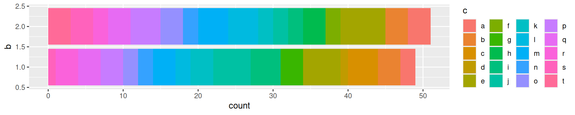

ggplot(sandbox.df, aes(x=b, fill=c)) + geom_bar() + coord_flip() +
  guides(fill=guide_legend(ncol=4)) + 
  scale_fill_manual(values=pal)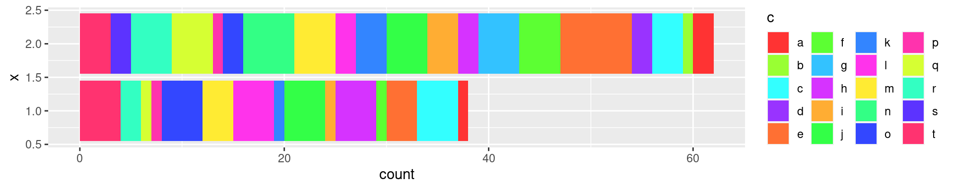

Another easy multi-color dark-ish palette is scales::muted(rainbow(N), l=60), with N the number of colors wanted (see example below).

Repel points/labels

To label points, even when they are crammed.

library(ggrepel)
library(dplyr)
zoom.df = sandbox.df %>% filter(x>.6) %>%
  mutate(label=ifelse(x>.9, paste('point', c, b, round(x,2)), ''))

ggplot(zoom.df, aes(x=x, y=x, label=label)) + geom_point() +
  geom_label_repel()

ggplot(zoom.df, aes(x=x, y=x, label=label)) + geom_point() +
  geom_label_repel(aes(label=label), max.overlaps=Inf,
                   nudge_x=sample(c(.01, -.01), nrow(zoom.df), TRUE)) +
  scale_x_continuous(expand = expansion(mult = .2)) + 
  scale_y_continuous(expand = expansion(mult = .2))

ggplot2 tricks

• To plot a density distribution without the x-axis line, use stat_density(geom="line") (and eventually position="dodge" if plotting several groups).
• To override the legend’s aes: guides(colour=guide_legend(override.aes=list(alpha=1)))
• Multi-column legends: guides(fill=guide_legend(ncol=4))
• Add more vertical space between legend labels (e.g. for multi-lines labels): guides(fill=guide_legend(keyheight=2))
• Don’t show a in legend when using text (e.g. when already having points and colors): geom_text(show.legend=FALSE)
• Keep “dodged” bars the same width: position=position_dodge(.9, preserve='single')
• Change direction of multi-legends: theme(legend.box='vertical')
• Remove some white space between legend and graph, or where the title used to be: theme(legend.margin=margin(-5))

Multi-panel ggplots

In general we can use grid.arrange. For example:

p1 = ggplot(...) + ...
p2 = ggplot(...) + ...
p3 = ggplot(...) + ...
grid.arrange(p1, p2, p3, heights=c(2,1), layout_matrix=rbind(c(1,1), 2:3))

p1 = p1 + ggtitle('A') + theme(plot.title=element_text(hjust=-.05, vjust=-3))

library(ggplot2)
library(gridExtra)
p1 <- ggplot(...
p2 <- ggplot(...
p1 <- ggplot_gtable(ggplot_build(p1))
p2 <- ggplot_gtable(ggplot_build(p2))
maxWidth = unit.pmax(p1$widths[2:3], p2$widths[2:3])
p1$widths[2:3] <- maxWidth
p2$widths[2:3] <- maxWidth
grid.arrange(p1, p2, heights = c(3, 2))

ggp.panels = grid.arrange(
    ggp.1 + theme(axis.text.x=element_blank(), axis.title.x=element_blank(),
                  plot.margin = margin(.1,.1,.1,.35, "cm")), 
    ggp.2 + theme(plot.margin = margin(.1,1.5,.1,.8, "cm")),
    heights=c(2,3))

Change font in ggplot2

library(extrafont)
font_import(pattern='Comic')
loadfonts()
qplot(x=rnorm(100)) + geom_histogram() + theme(text=element_text(family="Comic Sans MS")) + ggtitle('Ouch')

fonts() to check which fonts are imported by extrafont, names(pdfFonts()) to list the fonts available (loaded).

More in this blog post.

Waffle graphs

waffle package provides a waffle and iron function. For example:

iron(
  waffle(c(thing1=0, thing2=100), rows=5, keep=FALSE, size=0.5, colors=c("#af9139", "#544616")),
  waffle(c(thing1=25, thing2=75), rows=5, keep=FALSE, size=0.5, colors=c("#af9139", "#544616"))
)

Gantt charts

I used ganttrify for a grant. I tweaked the default output a bit to show a legend for the colors.

library(ganttrify)
library(ggplot2)
project = read.table('gantt.tsv', as.is=TRUE, header=TRUE, sep='\t')
## set the order of the activities from the order in the TSV file
project$wp = factor(project$wp, unique(project$wp))
spots = read.table('gantt-spots.tsv', as.is=TRUE, header=TRUE, sep='\t')
ggp = ganttrify(project=project, spots=spots,
                project_start_date="2024-01", month_breaks=6,
                mark_years=TRUE, hide_wp=TRUE, label_wrap=40,
                line_end = "butt", axis_text_align = "right") +
  theme(legend.position='top', legend.title=element_blank(),
        legend.margin=margin(0,100,-15)) +
  scale_color_brewer(palette='Dark2', breaks=unique(project$wp)) + 
  guides(color=guide_legend(ncol=3))
ggp 

Zoom-on-click images

To get this feature on an HTML report, add anywhere (or by including an html file e.g. with includes: before_body:)

<script src="https://ajax.googleapis.com/ajax/libs/jquery/3.1.1/jquery.min.js"></script>

<style>
.zoomDiv {
  opacity: 0;
  position:fixed;
  top: 50%;
  left: 50%;
  z-index: 50;
  transform: translate(-50%, -50%);
  box-shadow: 0px 0px 50px #888888;
  max-height:100%; 
  overflow: scroll;
}

.zoomImg {
  width: 100%;
}
</style>

<script type="text/javascript">
  $(document).ready(function() {
    $('body').prepend("<div class=\"zoomDiv\"><img src=\"\" class=\"zoomImg\"></div>");
    // onClick function for all plots (img's)
    $('img:not(.zoomImg)').click(function() {
      $('.zoomImg').attr('src', $(this).attr('src'));
      $('.zoomDiv').css({opacity: '1', width: '100%'});
    });
    // onClick function for zoomImg
    $('img.zoomImg').click(function() {
      $('.zoomDiv').css({opacity: '0', width: '0%'});
    });
  });
</script>

All the images can then be clicked on to display a zoomed in display. Click again on the image to close the zoomed image.

Note: It required pandoc version >2 to load the javascript lib.

Other options I haven’t tried yet:

• knitrBootstrap seems to include a similar feature by default.
• fancybox like described in this tufte issue.

Beamer presentation

Some useful options to put in the YAML header:

title: The Title
subtitle: The Subtitle
author: Jean Monlong
date: 11 Oct. 2016
output:
  beamer_presentation:
    slide_level: 2
    fig_width: 7
    includes:
      in_header: header.tex
    toc: true
    dev: png
    keep_tex: true

• slide_level defines the header level to be considered as a new slide.

To add slide count I put this on the header.tex:

\setbeamertemplate{navigation symbols}{}
\setbeamertemplate{footline}[page number]

```{r, include=FALSE}
knitr::knit_hooks$set(resize = function(before, options, envir) {
    if (before) {
      return('\\resizebox{\\textwidth}{!}{')
    } else {
      return('}')
    }
})
```

## Wide table

```{r, resize=TRUE}}
knitr::kable(matrix(rnorm(10),10,10), format='latex')
```

Jekyll website

The Rmd files located in the _source folder get automatically compiled by servr package using this command:

Rscript -e "servr::jekyll(script='build.R', serve=FALSE)"

Note: I now use blogdown which automatically compile the R Markdown documents (every page is a R Markdown actually).